
Models of Computation
13. Models of Computation
The first module of this course deals with the technical foundations of all digital systems, specialized to an endless variety of specific applications. For the remainder of the course, we refocus our attention on a particular class of digital system: the general purpose computer. The distinguishing feature of this class of digital systems is that their behavior is dictated by algorithms encoded as digital data, rather than being wired into the digital circuitry that constitutes their hardware design. This distinction represents a major conceptual revolution of the early $20^{th}$ century, and one that underlies modern computer science and engineering. Its immediate consequences are the conceptual distinction between hardware and software, the notion of programming and programming languages, interpretation and compilation as engineering techniques, and many other issues central to contemporary computer science. Fundamental ideas that underly this important paradigm shift are the topic of this Chapter. We may view these seminal ideas as the product of a search, during the first half of the twentieth century, for a suitable formal model of digital computation: a sound mathematical basis for the study of the universe of computational algorithms and machines capable of performing them. This Chapter marks our transition to this new focus by sketching foundational ideas of Computer Science resulting from that search.FSMs as a model of computation
13.1. FSMs as a model of computation
Finite state machines, described in Chapter 9, are an attractive candidate as a model of computation. We may view a simple ROM-based FSM as a programmable general-purpose (or at least multi-purpose) computation machine, in that its behavior may be modified simply by changing the string of bits stored in its ROM. Of course, any particular FSM implementation as a digital circuit necessarily fixes the number of inputs, outputs, and states as implementation constants, limiting the range of FSM behaviors that can be achieved by reprogramming its ROM.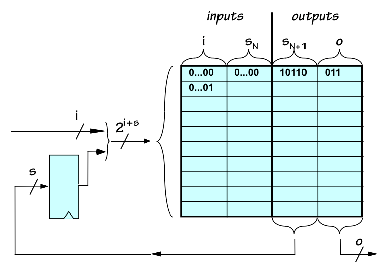
Generalized FSM implementation
FSM enumeration
13.1.1. FSM enumeration
Although the bound established by $FSMS(i,o,s)$ grows large as the parameters $i, o, s$ increase, we note that it remains finite for finite $i, o, s$. This observation suggests an intriguing conceptual exercise: we could define an infinite list that includes every possible FSM -- with some duplicates, due to equivalence -- by enumerating the possible ROM configurations for each set of $i, o, s$ values in some canonical order.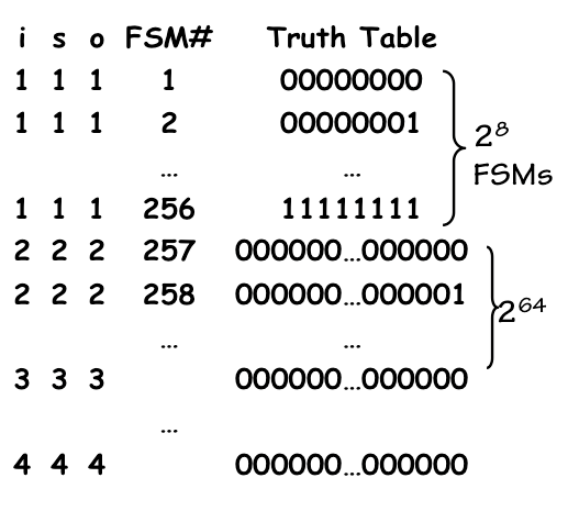
FSM Enumeration
FSMs as a Model of Computation
13.1.2. FSMs as a Model of Computation
The ability to conceptually catalog FSMs of all sizes, and consequently the set of computations that can be performed by FSMs of all sizes, makes FSMs attractive as a formal model for the computations we might perform by digital circuitry. Moreover, FSMs have been extensively studied and their formal properties and capabilities are well understood. For example, for every class of strings described by a regular expression -- a parameterized template including "wild card" and repetition operators -- there is an FSM that will identify strings of that class. For these reasons, finite state machines have become, and remain, an important formal model for a class of computations. A natural question arises as to whether FSMs are an appropriate formal model for all computations we might want to perform using digital circuitry. If every computation we might want a digital system to perform can be performed by some finite state machine, does this reduce the process of digital system engineering to the simple selection of an FSM from our enumerated catalog of possibilities? Of course, this extreme view ignores practical issues like cost/performance tradeoffs; however, the question of whether the class of computations performed by FSMs is a suitable abstraction for all practical digital computations is clearly worth answering.FSM limitations
13.1.3. FSM limitations
Although FSMs can clearly perform a variety of useful operations, there are simple, well-defined computations that cannot be performed by any finite state machine.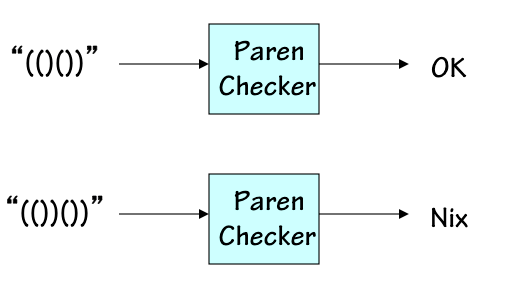
Paren Checker
Alternative Models
13.1.4. Alternative Models
The search for an abstract model of computation capable of dealing with a broader class of algorithms was an active research topic during the early $20^{th}$ century. Proposed candidates explored a wide variety of approaches and characteristics, and many have had lasting impact on the field of computer science. Examples include:- The lambda calculus of Alonso Church, simple model for functional programming languages;
- The combinatory logic of Schonfinkel and Curry, a model for functional programming without variables;
- The theory of recursive functions of Kleene;
- The string rewriting systems of Post and others, in which system state stored as a string of symbols evolves under a set of rewrite rules;
- Turing machines, discussed in the next section.
Turing Machines
13.2. Turing Machines
One of the alternative formalisms for modeling computation was a simple extension of FSMs proposed by Alan Turing in 1936.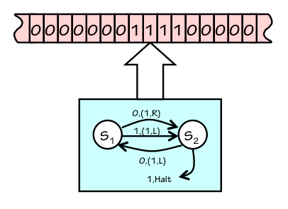
A Turing Machine
- Mounting a tape containing some initial configuration of 0s and 1s, with the tape head pointing to a appropriate starting point. This configuration encodes an input to the computation.
- Starting the Turing Machine (with its FSM in a designated inital state).
- Letting the Turing Machine run until its FSM reaches a special halting state.
- Reading the final configuration of 1s and 0s from the tape of the halted machine. This configuration encodes the output of the computation.
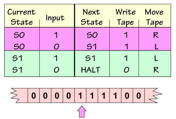
Unary Incrementor TM
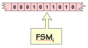
Turing Machine i
About that Infinite Tape
13.2.1. About that Infinite Tape
The use of an infinite tape certainly marks the Turing machine as a conceptual rather than a practical tool and may provoke some skepticism in the practical-minded reader. In fact our interest is in practical computations: ones that complete in a finite number of steps. Every such finite computation will visit at most a finite number of positions on the infinite tape: it will read finitely many positions as input, and write finitely many positions as output. So every finite computation -- every one of the practical computations in which we profess interest -- can be completed with a finite tape of some size. The difficulty that motivated us to consider Turing machines rather than FSMs is that we cannot put a finite bound on that size without restricting the set of functions that can be computed. A conceptually convenient way to relax that restriction is to simply make the storage (the tape) infinite. There are plausible alternatives to this abstraction mechanism. We might, for example, replace each Turing machine $TM_i$ by a family of finite-memory Turing machines $TMF_i^S$ with varying values of $S$, a finite tape size. The statement that "computable function $f_i$ can be performed by Turing machine $TM_i$" would then become "function $f_i$ can be performed by $TMF_i^S$ for sufficiently large S. We choose to duck this complication by the conceptually simple notion of an infinite tape. Do keep in mind, however, that every finite computation uses at most a finite portion of the tape: it will read and write at most some bounded region surrounding the initial tape head position.TMs as Integer Functions
13.2.2. TMs as Integer Functions
In order to compare the computational power of Turing Machines with alternative models such as those mentioned in Section 13.1.4, it is useful to characterize the computation performed by a given TM as an integer function -- that is, a function taking an integer input and producing an integer output. To do so, we adopt a convention for encoding a bounded tape configuration -- a configuration containing finitely many 1s (other positions containing 0) -- as a nonnegative number.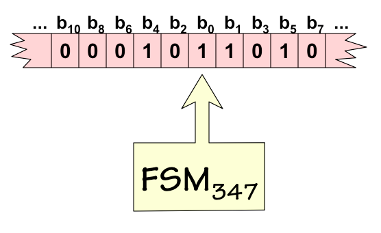
TM 347 on tape 51
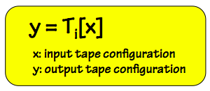
TM as integer function
Functions as Expressive Power
13.3. Functions as Expressive Power
Mathematicians studying these early models of computation used the set of integer functions computable by each model as a measure of that model's expressive power -- the idea being that if a given function (say, square root) could be expressed in one model but not in another, the latter model is less powerful in some mathematically significant sense. There ensued a period during which the set of integer functions computable by each of the proposed models was actively studied, partly motivated the desire to "rank" the proposed models by expressive power. It is worth noting that the set of integer functions in question can be generalized in various ways. Functions of multiple integer arguments can be encoded using integer pairing schemes -- for example, representing the pair $(x,y)$ of arguments to $f(x,y)$ as a single integer whose even bits come from $x$ and whose odd bits come from $y$. Similarly, representation tricks like those sketched in Chapter 3 can allow symbols, approximations of real numbers, and other enumerable data types to be represented among the integer arguments and return values of the functions being considered. These coding techniques allow us to represent a very wide range of useful computations using integer functions -- in fact, using single-argument functions defined only on natural numbers (nonnegative integers).An N-way tie!
13.3.1. An N-way tie!
The remarkable result of this attempt to identify the most expressive of the candidate models of computation, by the metric of expressibility of integer functions, was that each of the models studied could express exactly the same set of integer funtions. The equivalance of the models by this metric was proven, by showing systematic techniques for translating implementations in one model to equivalent implementations in another. For example, there is a systematic algorithm to derive from the description of any Turing machine a Lambda expression that performs precisely the same computation, implying that the expressive power of Lambda expressions is at least that of Turing machines. Moreover, there is an algorith for translating any Lambda expression to a Turing machine that performs the same computation, implying that Lambda expressions are no more expressive than Turing machines. This same set of integer functions may be implemented in many other computation schemes, a set including those mentioned in Section 13.1.4 and countless others, among them most modern computer languages.Church's Thesis
13.3.2. Church's Thesis
The discovery that the same set of integer functions is computable by every computation scheme of sufficient power that was studied strongly suggests that that set of functions has a significance that goes beyond the properties of any given model of computation. Indeed, it suggests that there is an identifiable set of computable functions that can be implemented by any sufficiently powerful computation scheme, and functions outside this set cannot be computed by any machine we might implement now or in the future.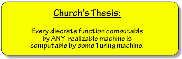
Computable Functions
13.3.3. Computable Functions
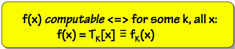
Computable Functions
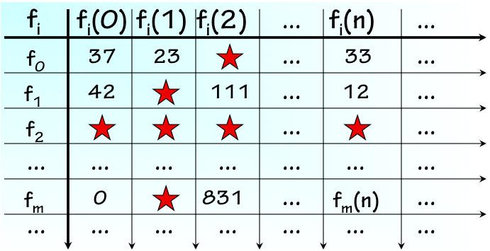
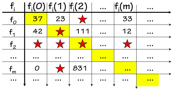
Enumeration of Computable Functions
The Halting Problem
13.3.4. The Halting Problem
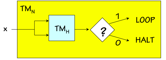
Given the range of useful functions performed by modern computers, each demonstrably implemented using computable functions, it may be surprising to the uninitiated reader that the majority of well-defined functions are in fact uncomputable. In this section we demonstrate an example of an uncomputable function. Consider the problem of determining whether Turing Machine $k$ will halt given input tape $j$ -- equivalently, whether the $k^{th}$ computable function applied to the argument $j$, $f_k(j)$, is well defined. It would be useful to have an effective implementation of this function, for example, if we were building a program to answer questions about values in the infinite table of the previous section.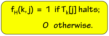
The Halting Function
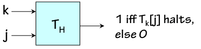
Halting TM
Universal Turing Machines
13.4. Universal Turing Machines
Given the correspondence between computable functions and Turing Machines, we face the prospect of a different Turing Machine design for every computable function we might wish to compute. Indeed, we might have different special-purpose physical machines to multiply, take square roots, or compute payroll taxes: each machine would consist of an application-specific FSM intefaced to an infinite tape. Each Turing Machine is a special-purposecomputer, whose application-specific behavior is wired into the design of its FSM. It seems clearly possible, however, to cut down on our inventory of special-purpose TMs by designing TMs capable of performing multiple functions. A single Turing Machine could certainly be capable of multiplying and taking square roots, depending on the value of an input devoted to specifying which function to perform. Indeed, a little thought will convince us that if functions $f_1(x)$ and $f_2(x)$ are both computable, then the function \begin{equation} f_{1,2}(x,y) = \begin{cases} f_1(x), & \mbox{if } y = 1 \\ f_2(x), & \mbox{if } y = 2 \end{cases} \end{equation} is also computable. Our Church's Thesis insight convinces us that, given physical machines that compute $f_1$ and $f_2$, we could build a new machine that computes $f_1$ or $f_2$ depending on the value of a new input. More formally, we could (with some effort) demonstrate an algorithm that takes the state transition diagrams of FSMs for two arbitrary Turing Machines $TM_i$ and $TM_j$, and constructs the diagram for a new $TM_{i,j}$ capable of behaving like either $TM_i$ or $TM_j$ depending on an input value. If a single Turing Machine might evaluate any of several computable functions, is it possible that a single Turing Machine might be capable of evaluating every computable function? We can formalize this question by formulating a simple definition of a universal computable function $U(k,j)$ as follows: $$U(k, j) = TM_k(j)$$ This Universal function takes two arguments, one identifying an arbitrary Turing Machine (hence an arbitrary computable function) and a second identifying an input tape configuration (hence an argument to that function). It returns a value that is precisely the value returned by the specified Turing Machine operating on the given tape: the computation $U(k,j)$ involves emulating the behavior of $TM_k$ given tape $j$. The existence of a TM capable of evaluating every computable function now amounts to the question of whether $U(k,j)$ is a computable function: if it is, then by our definition it is computed by some Turing Machine, and that machine is universal in the sense that it can compute every function computable by every Turing Machine. Given our discovery that the majority of functions are (sadly) not computable, we might be pessimistic about the computability of $U(k,j)$. Remarkably, however, $U(k,j)$ is computable. There are in fact an infinite number of Turing Machines that are universal in the above sense. Each universal machine takes input that comprises two segments:- A program specifying an algorithm to be executed (argument $k$ of $U(k,j)$); and
- Some data that serves as input to the specified algorithm (argument $j$ of $U(k,j)$).
Turing Universality
13.4.1. Turing Universality
Universal Turing Machines have the remarkable property that they can mimic the behavior of any other machine, including that of other universal Turing machines, at least by the measure of the functions they can compute. That measure seems to capture their computational scope, although it ignores dimensions of their power like performance and details of I/O behavior. A universal Turing machine without audio output hardware cannot play audio, for example, although it can compute a stream of bits that represents a waveform to be played. Of course, not every Turing machine is universal; the Unary Incrementor of Section 13.2, for example, cannot mimic the computational behavior of an arbitrary Turing machine. The distinction between machines that are universal in the Turing sense and those that are not has emerged as a basic threshold test of computational power. It is applicable not only to Turing machines, but to arbitrary models of computation -- including computer designs and programming languages. A programmable device or language that is Turing Universal has the power to execute any computable function, given the right program. By this standard, it is at the limit of computational power.Interpretation
13.4.2. Interpretation
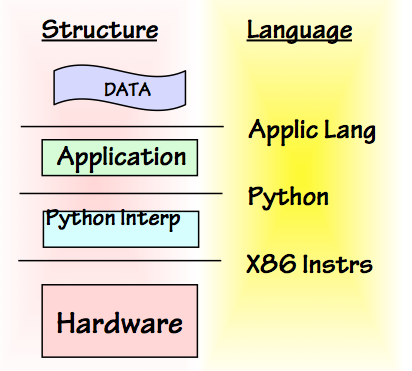
The ability of a universal machine to mimic the behavior of another machine is the basis for a powerful engineering abstraction mechanism, one that underlies the field of Computer Science. That mechanism is the interpretation of a coded algorithm -- a program -- to effect the execution of that algorithm. Imagine, for example, we have a simple universal machine $M1$ which is easy to manufacture but difficult to program due to its primitive nature. The language $L1$ accepted by $M1$ for its programs passes the universality test, but may require every operation to be expressed in terms of single-bit NANDs rather than (say) arithmetic operations.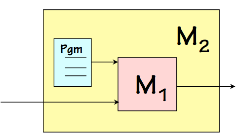
Interpretation

Layers of Interpretation
Language Interfaces
Compilation
13.4.3. Compilation
The preceeding examples show interpretation as a mechanism for moving from one interface language to another -- for example, for executing Python programs on a machine that can execute X86 machine language. There is an alternative mechanism for this language-level mobility, also commonly used in modern systems, that is subtly different from interpretation: we refer to it as compilation. While interpretation involves emulating the behavior specified by an encoded algorithm, compilation involves translating an algorithm from one language to another.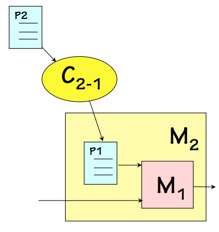
Compilation
- what: Interpreters and compilers both take a progrogram as input; however, the interpreter produces behavior as a result, while the compiler produces another program.
- where: The interpreter runs on the target machine (hence must be coded in the language of that machine); the compiler can run on any machine, and may hence be coded in an arbitrary language.
- how often: Interpretation is a mechanism for execution, and takes place whenever the interpreted program is executed. Compilation is a single translation step that yields a program that can be run (without re-compilation) many times. For this reason, compilation is typically more time-efficient for programs that are executed many times.
- when: Interpreted code makes implementation choices while the program is being executed (at "run time"); compilers make certain choices during the preliminary translation process ("compile time").
Context: Foundations of Mathematics
13.5. Context: Foundations of Mathematics
The foundational ideas of computer science discussed in this Chapter arose during a period in which a number of eminent mathematicians were preocccupied with the project of putting the field of mathematics itself on a logically sound conceptual basis. We sketch some landmarks of this history below:- Set theory as a basis for Mathematics:
- During the $19^{th}$ century, the idea emerged that all of mathematics could be based on set theory. This is not the set theory involving sets of apples and oranges that many of us encountered in our early education; rather, the pure mathemeticians espousing this view wanted to avoid postulating arbitrary concrete artifacts (like apples -- or for that matter numbers) and construct all of mathematics from a set of basic principles, namely the handful of axioms defining set theory. What concrete things can one construct from the axioms of set theory and nothing else? Well, we can construct the empty set. This concrete artifact gives some meaning to the notion of zero, the number of elements in the empty set. Given this first concrete artifact, you can make a set whose single element is the empty set, giving meaning to $1$ as a concrete concept. Following this pattern, one can build $2$, $3$, and the entire set of natural numbers. Additional conceptual bootstrapping steps lead to rationals, reals, and complex numbers; eventually, it can provide the foundations for calculus, complex analysis, topology, and the other topics studied in mathematics departments of contemporary universities.
- Russel's Paradox:
- At about the start of the $20^{th}$ century, Bertrand Russel observed that a cavalier approach to set theory can lead to trouble, in the form of logical inconsistencies in the theory being developed as the basis of all mathematics. Logical theories are frail, in that introduction of a single inconsistency -- say, $5 = 6$ -- gives them the power to prove any formula independent of its validity. For a formula $X$, an inconsistent logic could be used to prove both $X$ and not $X$, defeating its usefulness in distinguishing valid from invalid formulae. Russel's famous example of ill-formed sets involved the village barber who shaves every man who doesn't shave himself -- a homey proxy for a set containing all sets not contaning themeselves. Does such a set contain itself? Either answer leads to a contradiction, revealing an inconsistency in set theory. Other Russel folklore includes his public assertion that any inconsistency allows every formula to be proved, prompting a challenge from the audience for Russel to prove himself the Pope given the assertion that $5=6$. The story has Russel accept and elegantly fulfill that challenge.
- Hilbert's Program:
-
While the set theoretic pitfall observed by Russell was
fairly easy to sidestep, it raised an important issue:
how can we be sure that all of mathematics is in fact
on a sound basis? It would be disasterous for centuries
of mathematicians to prove new results, only to find that
each of these results could be disproved as well due to
an undetected inconsistency in the underlying logic assumed.
A number of mathematicians, famously including David Hilbert,
undertook a program to assure mathematics a provably sound
basis.
Their goal was to establish an underlying logic which was
simultaneously
- consistent, meaning that only valid formulae could be proved; and
- complete, meaning that every valid formula can be proved.
- Gödel's Incompletness Theorm:
- In 1931, the Austrian mathematician Kurt Gödel shocked world of mathematics and shattered the lofty goals of Hilbert's program. Gödel showed that any logical theory having the power to deal with arithmetic contains a formula equivalent to the English sentence "this statement can't be proved". A moment's reflection on the logical validity of this sentence reveals a problem: if it can be proved, the statement is false; hence the theory is inconsistent, allowing the proof of a false statement. If on the other hand it cannot be proved, the statement is true and the theory incomplete: there is a valid formula that cannot be proved. In this monumental work, Gödel pioneered many of the techniques sketched in this Chapter -- including enumeration (often called Gödel numbering in his honor) and diagonalization. It establishes that every sound logical theory of sufficient power contains unprovable formulae: there are bound to be true statements that cannot be proven. Gödel used the power of mathematics to circumscribe the limits to that power itself.
- Computability:
- In the wake of Gödel's bombshell, Turing, Church, and others showed that not all well defined functions are computable. Indeed, Turing showed moreover that not all numbers are computable by an intuitively appealing measure of computability. This succession of negative results during the 1930's challenged the field of mathematics as the arbiter of rational truth.
- Universality:
- Interspersed among these demonstrations of the limits of mathematics was the discovery that the tiny minority of functions that are computable comprises a remarkably rich array of useful computations. Of particular interest -- at the time, in a theoretical sense -- was the discovery that the universal function of Section 13.4 is in theory a computable function.
- General-purpose Computing:
- The universal Turing machine remained a conceptual experiment for a decade, until researchers began exploring the construction of practical machines based on the idea. Conspicuous among these was John von Neumann, whose landmark 1945 paper sketched the architecture of a machine design that has become recognised as the ancestor of modern general-purpose computers. Since the articulation of the von Neumann architecture, many profound conceptual and technology developments have driven the computer revolution. These include core memory, the transistor, integrated circuits, CMOS, and many others. But the basic plan for a stored-program general purpose computer, detailed in the next Chapter, has clear roots in von Neumann's vision and the universal function on which it is based.
Chapter Summary