14. Instruction Set Architectures

In this Chapter, we begin the transition of our focus from the engineering of digital systems in general to the engineering of contemporary general purpose computers, the practical embodiment of the universal Turing machines of Section 13.4.

The universal TM was intended as a conceptual tool -- a thought experiment rather than a proposal for a practical implementation. In practical terms, it suffers from at least three difficulties:

1. Infinite hardware: an infinite tape as its main storage resource.
2. Performance limitations: including bit-serial computations, long access times for distant memory locations on the tape.
3. Programming model: An unconstrained string of 1s and 0s on a tape provide a poor programming interface for building and maintaining large, modular software systems.

While the first two of these issues are fairly obvious, the last is a bit more subtle. Our desire to structure programs to reflect structure of a problem -- for example, to be able to simply construct a program that computes $f(g(x))$ from two programs that compute $f(x)$ and $g(x)$ respectively -- requires some discipline in the design of the programming interface itself.

14.1. Steps toward a General Purpose Computer

We naturally tend to view algorithms for practical computations as sequences of operations: each algorithm is a recipe outlining a series of sequential steps to be followed. There may of course be conditionals and loops, as shown in the sample program to the right; but the code describes finite sequence of operations such as $a \leftarrow a \cdot b$ replacing the value of some variable $a$ with the product of the values $b$ and $c$. This C program computes $N!$ using a loop that is executed as the variable $b$ is counted down from $N$ to $0$, accumulating in $a$ the product of all nonzero values of $b$ along the way.

14.1.1. Datapath vs. Control Circuitry

We might express the logic that orders the exection of the steps in this program execution as an FSM like that on the left. A starting state initializes the $a$ and $b$ variable values, after which the loop state is executed so long as $b \neq 0$. At each looping step, $a$ is replaced by a new $a \cdot b$ product and $b$ is counted down, escaping the loop when $b = 0$. Once completed, our FSM halts with the answer -- $F!$ -- in $a$.

To complete the construction of a factorial computer, we need to augment this FSM with the circuit for a datapath, controlled by our FSM, that implements the operations to be performed at each step. The datapath might contain two registers to hold values of $a$ and $b$, allong with operators that perform multiplication and decrementing required by our algorithm. Note that we have chosen to represent $a$, $b$, and $N$ as 32-bit unsigned binary values; hence the widths of data lines within our data path are 32 bits.

Our data path uses two 3-way multiplexors to select, on each clock cycle, inputs for the $a$ and $b$ registers. The select inputs to these multiplexors we view as control signal inputs to the datapath: inputs, generated by our separate control FSM, that control the operations and flow of data around the data path diagram.

The control FSM itself, shown to the right, is a simple clocked 3-state FSM whose state transition diagram is shown above. It has as its single input the 1-bit $z$ value from the data path indicating whether the contents of $b$ are zero. The ouputs of the FSM are the control signals required by the data path, viz. the select inputs for the two multiplexors. Logic for the control FSM, derived from the state transition diagram, is shown to the left.

The decomposition of a system into control and data path subsystems is a common technique for structuring complex digital systems, and one that we will follow in the processor design of Chapter 18.

14.1.2. Generalizing Datapath Design

The ad-hoc datapaths sketched in the above example could be generalized to allow a modestly wider range of computations to be implemented by modifying the logic of the control FSM. Consider for example the data path to the left, offering a set of four registers (labeled $R10$ through $R3$) and repertoire of four possible operations (sum, difference, product, and bitwise NAND). During each clock cycle, two source operands are selected from among the contents of the four registers via $a_{SEL}$ and $b_{SEL}$, and one the output of one of the four operators is selected by the $OP_{SEL}$ control signal. The result of the selected operation can optionally be routed to one destination regiser selected by the $W_{SEL}$ signal. The single input to the control FSM is the result of an equality test between the contents of the two selected source registers.

This enhanced data path design can be used to compute factorial as well as a number of other interesting functions. Of course, further enhancements are possible: a greater number of registers may be offered, as well as a larger repertoire of operations. Indeed, early multi-purpose machines similar to this design were constructed and used during the 1940s. Their programming typically involved setting myriad switches, establishing the logic of their FSM controller.

14.2. von Neumann Architecture

The multi-purpose architectures of the 1940s fail the test for Turing universality of Section 13.4.1, for at least two simple reasons:

1. A finite bound on the size of their control logic, hence on the complexity of the "program" to be executed;
2. A finite bound on the amount of data that can be stored during the course of their computation.

Both of these finiteness limitations are avoided by the infinite tape of the universal Turing machine, whose use for both program and data allows the two issues to be resolved by a single infinite resource.

In 1945, John von Neumann articulated a plan for building general-purpose computers that has become known as the von Neumann architecture and remains the rough blueprint for general purpose computers to this day. Major components of the von Neumann architecture include

• a Central Processing Unit or CPU, comprising logic that performs actual computation;
• a Main Memory used to store both data and coded instructions that constitute a program for processing that data; and
• an Input/Output component for communicating inputs and results with the outside world.

This plan may be loosely viewed as a pragmatic adaptation of the Universal Turing Machine. Main memory serves the function of the Turing machine's infinite tape, storing both programs (coded as sequences of instructions) and data. Although the size of main memory is finite, its size is viewed as a parameter of the implementation: in theory, it can be expanded to whatever finite size is required by the current computation. As noted in Section 13.2.1, such parameterization offers a practical alternative to making memory infinite.

The CPU performs roughly the function of the FSM of a Turing machine, reading instructions from main memory and executing them, accessing data from memory in the process.

The I/O provision of the von Neumann architecture an embellishment over the starkly minimalist approach to I/O used by Turing machines, which requires the infinite tape to double as the sole I/O device. The von Neumann plan anticipates dedicated I/O devices such as keyboards, displays, and bulk storage.

14.2.1. The Stored-Program Computer

The use of a single memory subsystem to store both programs and data, inspired by the tape of the Universal Turing Machine, constitutes a major difference between von Neumann's proposal and prior special-purpose computers whose computational function was wired into their circuitry. The von Neumann machine uses a single main memory, capable of holding a finite number of $W$-bit words of data, where the word size $W$ is a parameter of the architecture while the total main memory size is a parameter of the implementation. For example the IBM 360 (an influential architecture introduced in the 1960s) dictated a 32-bit word size and a specific instruction set, shared by all machines of the family. However, specific IBM 360 computers might have memory sizes varying from thousands to millions of words, depending on the budget and requirements of the customer.

It is conventional to identify each $W$-bit storage location in main memory with a unique address, typically an integer ranging from 0 to the total number of words of main memory. We can thus view main memory as a table of binary values as shown to the right, each of whose entries represents a location containing a word of data. In modern computer architectures the the word size $W$, as well as the number of bits in an address, are both typically powers of two. Often they are the same: thus an architecture whose word size is 32 bits will typically restrict main memory addresses to 32 bits as well - an architectural constraint that has been responsible for the obsolescence of many once popular architectures.

14.2.2. Anatomy of a von Neumann Computer

Although there are boundless ways to approach the implementation of a CPU, a good choice is the separation of the design problem using roughly the datapath versus control partitioning of shown to the right. This diagram teases the datapath portion of the CPU, containing logic for performing arithmetic and other operations on data, apart from the control portion that interprets instructions fetched from main memory and generates control signals for the datapath. Each of these two CPU subsystems needs an interface to main memory: the datapath needs to load and store data values, while the CPU needs to fetch coded instructions to be executed.

14.2.2.1. CPU Datapath

The datapath portion of the CPU typically includes some modest amount of internal storage, often in the form of a set of general-purpose registers each capable of holding a word of data. These registers serve as both sources and destinations of data for the simple arithmetic and logical operations performed by each coded instruction, using a datapath approach similar to that sketched on the right. In this datapath, control signals (generated by the control subsystem from a fetched instruction) include asel and bsel, which select two source data words as input to the ALU; a function code to specify the operation to be performed by the ALU; and dest, dictating a destination register into which the resulting value will be loaded.

14.2.2.2. CPU Control

The control circuitry of the CPU includes a modest amount of storage, to maintain its state; typically this consists primarily of a program counter or PC, a register capable of holding an arbitrary main memory address. The contents of the program counter specify the main memory address containing the next coded instruction to be executed by the CPU. Each instruction encodes the operations to be performed, as well as the locations of source (input) and destination (output) operands, typically both registers within the datapath. With certain exceptions, the CPU increments the contents of the PC after the execution of each instruction, effecting the execution of a sequence of instructions stored in consecutive locations of main memory. 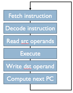The control of a typical von Neumann CPU roughly comprises the steps of the flow diagram to the right, a fetch/execute loop that fetches and executes a stream of single instructions in some prescribed sequence. The main memory location of the next instruction to be executed is stored in the program counter, which is updated after every instruction execution. Because of their sequential execution of a single stream of instructions, such CPUs are sometimes refered to as single-sequence machines, distinguishing them from processors capable of executing multiple instructions concurrently.

14.3. Instruction Set Architecture as an Abstraction

Before diving into the detailed specification of our example stored-program instruction set, it is worth reflecting on the design of an instruction set architecture or ISA as an engineering problem.

An instruction set architecture specifies how programs are to be encoded for a family of computers sharing that architecture. Once coded in a specific ISA, a program can generally be run on various machines sharing that ISA provided sufficient memory and I/O resources are available. In this respect, an ISA is an important engineering abstraction: it specifies an interface between hardware and software, and -- like other engineering abstractions -- allows both technologies to evolve independently.

The design of an instruction set is subject to a number of pressures:

• Cost/performance. It is clearly desireable that an ISA be cheap to implement and execute programs quickly.
• Cost/performance scaling. A related, more subtle goal is that the ISA be consistent with implementations over a wide range of the cost/performance spectrum; that is, allowing specific programs to be run quickly on expensive computers or more slowly on cheaper ones.
• Model of computation. During much of the history of general-purpose computing, an ISA design often reflected a particular language family or computation model: machines were designed around, say, ALGOL or LISP.
• Backward compatibility. Common ISA desiderata include the requirement that a new architecture be able to run dusty deck software written for now-obsolescent machines.
• Future compatibility. Forward-looking ISAs are designed to anticipate new trends in both hardware and software, often by providing an evolutionary path for the ISA itself.

Each of these goals represents an engineering challenge; satisfying each involves some cost, and different chapters of the evolving computer engineering technology have led to successive trends in ISA design. Well-designed ISAs, like the IBM 360, have been spectacularly successful as engineering abstractions by allowing the same software to be run on many computers spanning a wide range of cost/performance tradeoffs and decades of technology advances.

The isolation of software compatibility from technology-dependent hardware details remains a major goal in the design of instruction sets. In recent decades, however, it has been increasingly popular to downplay ISA details as the key to this compatibility, viewing instead some relatively machine-independent compiled language (such as C) as the interface specification. This view, popularized by Patterson and Hennessey as part of the Reduced Instruction Set Computer (RISC) movement, argues for starkly simplifying instruction sets by eliminating ISA "baggage" whose performance impact on the execution of real programs cannot be demonstrated by actual or simulated execution.

The appeal of this RISC argument stems in part from the Turing universality of the general purpose machines for which we are designing ISAs. Each general purpose machine can perform the same computations, which we can specify in a reasonably machine-independent way using a higher-level language than machine instructions. So why not use our body of existing software as benchmarks, and tune the ISA design to maximize performance? Such thinking has been a major driver for ISA evolution over recent decades, resulting in steady, incremental progress in the design and implementation of ISAs.

One plausible danger in this quantitative hill climbing approach to ISA evolution is that its basis on existing benchmarks may miss architectural innovations that require a new, alternative programming discipline: existing programs are optimized, to varying extents, to existing ISAs. It is possible that certain radical ISA improvements will require radically different software structures to demonstrate their advantages.

14.4. The Beta: An Example Instruction Set Architecture

To facilitate concrete examples throughout the remainder of this course, we introduce a simple but representative instruction set architecture called the Beta (a name inspired by the Alpha architecture of the now-defunct Digital Equipment Corporation). The Beta's ISA and programming model will be described in remaining sections of this Chapter and Chapter 16; two different implementations will be the subjects of Chapter 18 and Chapter 20.

The Beta ISA is a representative 32-bit RISC design, and lends itself to implementation strategies similar to that sketched in Section 14.2.2. The programmer-visible state of the CPU is stored in a set of general-purpose registers and a program counter.

14.4.1. Beta CPU State

The programmer-visible state of a Beta CPU includes a 32-bit program counter (PC) and a set of 32 general-purpose registers, each holding 32 bits. We distinguish programmer-visible state from other storage that may be hidden within a Beta implementation; remember that an ISA is an engineering abstraction, designed to allow various different implementation strategies.

The pool of general registers are intended to be used for various purposes dictated by the running software, e.g. to hold data relevent to the computation currently being performed. We number them consecutively from $0$ through $31$, and refer to them in text and programs as $r0$ through $r31$.

Register $r31$ is a special case whose contents are always a 32-bit word of zeros. This special case serves as a ready source of the constant zero as well as a destination for data to be discarded. The remaining registers, $r0$ through $r30$ are functionally identical from a hardware standpoint, although shortly we will establish software conventions for the use of certain of them.

14.4.2. Byte Addressing

The main memory of the Beta consists of an implementation-dependent number of 32-bit locations as described in Section 14.2.1, with one important additional complication: a unique address is assigned to each 8-bit byte in memory, rather than to each 32-bit word. This byte addressing scheme was introduced in the 1960s in the IBM 360 ISA, and remains popular among current architectures.

As a consequence of byte addressing, the main memory addresses of consecutive words differ by four rather than by one, since there are four 8-bit bytes in each 32-bit word. Squandering addresses in this way affords the option of addressing individual bytes within a word, say to deal conveniently with character strings stored as sequences of 8-bit character codes. While we will not implement byte-level addressing in our Beta hardware, some machines (like the IBM 360) have done so.

14.4.2.1. Endian Battles

The advent of byte addressing stimulated a famous and costly battle within the computer industry, dubbed the Endian battle in a tongue-in-cheek article by Danny Cohen. The issue arises on machines that allow both individual bytes and 32-bit words to be addressed within the same memory. The 32-bit word stored at location 0 comprises four bytes, whose addresses are 0, 1, 2, and 3; but which portion of the 32-bit word addressed as byte 0?

There are two obvious answers to this question: byte 0 is the high-order byte of the 32-bit word, or its the low-order byte. Although in retrospect the industry could have done fine using either convention, manufacturers split quite evenly between the two options: DEC and Intel, for example, used the little endian (byte 0 is low order) convention, while IBM and Motorola chose the opposite big endian byte order (until IBM chose to use Intel processors in its PC product line). This lack of standardization of byte ordering extends beyond ISA design to representation of multi-byte data in shared data structures and network communications, complicating interface specifications and communication.

While proponents of each byte ordering convention once defended their choice with religious zeal, it is generally recognized today that, aside from backwards compatibility issues, the advantages of either choice are outweighed by the costs of inconsistency among the industry.

14.5. Notation: Register Transfer Language

In order to describe sequences of computation steps in a relatively ISA-independent way, e.g. for documenting the semantics of individual instructions, we use an informal register transfer language (RTL).

R0 ← Mem[0x100]
tmp ← R0 + 3
Mem[104] ← tmp | 0x7

The sample RTL shown to the left specifies a sequence of computational steps, one corresponding to each line of the pseudocode. Each step involves an transfer of a value specified by the expression to the right of the ← operator to a destination specified by the expression to the left of the ←. Source expressions may involve constants, main memory locations (designated in the form Mem[address], or register names like R0 or PC. Destinations may be variable names, memory locations, or registers.

14.6. Programming Conventions: Storage Use

The design of an instruction set architecture reflects, to a great extent, the set of programming conventions it is intended to support. Modern programming involves a basic set of common constructs such as variables, expressions, procedures, and loops that need to be supported efficiently.

int x, y;
y = x * 37;

Consider, for example, the 2-line snipped of C code on the right. The first line declares two variables, x and y; the second line assigns a new value to y computed from the current value of x.

Like most contemporary computer systems, we choose a systematic strategy for representation of variables and the evaluation of expressions involving them. In particular:

• For every variable, we assign a location in main memory to hold a representation of its current value.
• Instructions operate on operands in general registers, which are used to hold for short-term copies of variable and other temporary values.
• Computations involving variables requires (1) loading the variable values from main memory into registers, (2) performing the computation using values in registers, and then (3) storing results back into the main memory locations assigned to effected variables.

Following this model, the declaration of the variables x and y in the snippet of C code above would cause each to be assigned a main memory address, perhaps at hex addresses 0x1008 and 0x100C in a region of memory reserved for variable storage. Note that each variable is assigned a full four byte (32-bit) storage location, since our chosen run time representation of an integer variable requires 32 bits. Given byte addressing, this implies that addresses of such variables stored in consecutive memory locations differ by four.

In order to effect the assignment statement y = x * 37; of our C code snippet, we need to (1) load the value of x into a register, (2) multiply it by 37, and (3) store the result into the main memory location assigned to y.

R0 ← Mem[0x1008]
R0 ← R0 * 37
Mem[100C] ← R0

Choosing arbitrarily general register 0 from the pool of registers available in our datapath for temporary use, we can effect the three required steps as shown in the RTL to the right. A remaining task is to specify how operations like the three steps in the given RTL can be encoded as Beta instructions.

14.7. Instruction Coding

A major portion of an Instruction Set Architecture specification deals with the repertoire of instructions provided by compliant machines, and details of their encoding as binary contents of locations in main memory. An understanding of the representation of instructions and their interpretation by the machine constitutes the programming model presented by the machine: a specification of the machine language that constitutes the most basic hardware/software interface presented by that machine.

Approaches to coding of machine instructions are subject to the engineering pressures mentioned in Section 14.3, and have evolved with hardware and software technologies over the history of the von Neumann architecture. Aspects of this evolution include

• Complexity: Certain historically successful instruction sets -- including the IBM 360 and DEC VAX -- offer a rich repertoire of high-level instructions to perform relatively complex computations within a single instruction. As an example, the VAX has a single instruction whose execution evaluates an arbitrary single-variable polynomial for a given value of its variable. Such complex instruction sets -- derisively called CISC in contrast to the simpler RISC approach popularized in the 1980s -- typically demanded a simpler machine language (called microcode) hidden within the hardware that interprets the complex machine language advertised by the ISA. RISC ISAs, like the Beta, offer a limited set of basic operations as single instructions, depending on sequences of such instructions to perform more complex computations.
• Instruction size: A related issue is the number of bits used to encode a single instruction. Many CISC ISAs have variable-length instructions, allowing simple operations to be performed by short instructions (e.g. one or 2 bytes of memory) intermixed with longer instructions encoding elaborate computations. While this feature offers flexibility to encode a wide variety of operations as single instructions, it complicates instruction fetch and decoding, making certain performance improvements (such as the pipelined execution of Chapter 20) impractical. The Beta ISA takes the typical RISC route of using a single 32-bit word to encode each instruction.
• Access to main memory: Some ISAs support enconding of single instructions that perform operations (like addition) of operands stored in main memory, which requires somehow encoding their main memory locations within the instruction itself. Others, like the Beta, restrict such operations to operands in CPU registers, and provide separate instructions to move data between registers and main memory.
• Access to constants: Common computations often involve constants: you need $\pi$ to compute the area of a circle from its diameter, and 6 to compute to compute the number of ounces in a sixpack. Given that an ISA needs the ability to access the value of variables stored in main memory, constants might simply be implemented as variables that are initialized to the appropriate value and never changed. But this approach involves time and program size costs for every use of a constant; consequently, instruction sets commonly provide a simple way of embedding short instruction-stream constants directly in certain instructions to avoid the overhead of additional memory accesses. The Beta provides instructions containing short (16-bit) constants.

There are many other such tensions between ISA design choices and technology -- both software and hardware -- that surface as we consider implementation strategies.

14.8. Beta Instructions

As suggested by the previous sections, the Beta ISA offers three general classes of instructions:

• Operate class instructions: encode an ALU operation to be performed on operands held in general registers within the CPU.
• Memory access instructions: Load CPU registers from and store registers to locations within main memory.
• Flow control instructions: By default, the Beta program counter is incremented (by 4, due to byte addressing) after each instruction is fetched; hence its default operation is to execute a sequence of instructions stored at successively increasing word addresses in main memory. The flow control insructions allow this sequential execution default to be varied; they change, perhaps conditionally, the contents of the program counter and hence the next instruction to be executed. They provide for programmed loops, branches, conditional execution, and procedure calls.

All Beta instructions are encoded as 32-bit words. Each instruction is encoded in one of two similar formats, shown to the right; in each case, the 32 bits of the instruction comprise four shorter fields, each specifying an independent parameter of the instruction. The fields are

• OPCODE: bits 26 through 31 of every Beta instruction. The value stored in this 6-bit field dictates what operation is encoded by the instruction, including which of the three instruction classes it represents and which of the two formats are used for the remaining bits of the instruction.
• Rc: bits 21-25 of every Beta instruction. This 5-bit field encodes the "name" of a register (meaning a number from 0 through 31 identifying one of the 32 CPU registers). It is used to encode a destination register for an operation, i.e., which register is to receive the result computed by that instruction.
• Ra: bits 16-20 of every Beta instruction. This 5-bit field encodes another register, typically the register containing a source operand to be used as an input to the operation performed by the instruction.
• Rb: bits 11-15 of Beta instructions using the first instruction format. This 5-bit field encodes another register, typically containing a second source operand.
• literal: bits 0-15 of Beta instructions using the second instruction format. This 16-bit field replaces the Rb field of the first format, and holds a 16-bit instruction-stream constant. Among other uses, it provides for operations (like ADD) in which one operation is a small constant.

14.8.1. Encoding Binary Operations

The largest class of instructions in the Beta ISA are those that perform actual computation: binary arithmetic, comparisons, and bitwise logical operations on data stored in CPU registers. In a typical Beta CPU, these operations are performed in an Arithmetic Logic Unit (ALU) that takes two 32-bit binary operands as input, along with a function code specifying the operation to be performed, and produces a single 32-bit binary result.

Using our first instruction format, we can encode an operation by choosing an appropriate opcode (which identifies the operation as well as the instruction format), and filling the three register-name fields to specify two source and one destination registers.

For example, a Beta instruction to add the contents of registers R1 and R2 and place the result in R3 would be encoded as shown to the right. The leftmost field of the instruction, its 6-bit OPCODE, is filled with a binary operation code assigned to the ADD operation. The next $r_c$ field contains the 5-bit "name" (binary number 3) of the destination register R3 that is to be loaded with the result of the operation. The remaining two 5-bit fields, $r_a$ and $r_b$, indicate source registers R1 and R2 whose contents are the values to be added.

14.8.2. Notation: Symbolic Instructions

It is convenient to have a textual symbolic representation for machine instructions; we use the notation ADD(R1,R2,R3) to designate the Beta instruction encoded with the ADD opcode, and 1, 2 and 3 in the respective fields $r_c$, $r_a$, and $r_b$. As elaborated in Section 15.2, this representation is an example of the assembly language we will use as the lowest-level programming interface to Beta processors.

We might document the semantics of the ADD instruction by associating the symbolic representation of its encoding with an RTL description of the resulting execution: ADD(Ra,Rb,Rc): Reg[Rc] ← Reg[Ra] + Reg[Rb]

14.8.3. Beta Operate Instructions

There is a modest repertoire of binary arithmetic and logical operations that neatly fit the same pattern as the ADD instruction. Each of these has a corresponding operate-class Beta instruction, with its unique opcode. These instructions are summarized below: In addtion to familiar arithmetic operations on binary integers, the Beta provides bitwise logical operations on 32-bit binary words, signed integer comparisons, and shifts. This set of operations corresponds roughly to the operators available in expressions in popular high-level languages like C and Python; the op column of the table gives typical operator syntax in these languages.

Note that any of the 32 Beta registers can be specified for any of the operands of these instructions, including the special R31 whose contents are hard wired to the value zero. This leads to some useful special cases; for example,

• ADD(Rx, R31, Ry) adds the (zero) contents of R31 to Rx, storing the result in Ry. It effectivly copies the value from Rx to Ry.
• ADD(Rx, Ry, Rx) increments the value in Rx by the value in Ry. It is important to note that the source operands get the values in the registers prior to the execution of the instruction, not (in this case) the updated value being stored back into Rx.
• ADD(Rx, Rx, Ry) doubles the value in Rx, storing the result in Ry.
• ADD(Rx, Ry, R31) computes the sum of its two source operands, but stores the result in the always-zero R31 -- effectively discarding the result. This is an example of a no-operation (or NOP) instruction, whose execution has no visible effect on the CPU state beyond incrementing the PC.

14.8.3.1. 32-bit Arithmetic and Overflow

The Beta ISA includes the four basic arithmetic operations, each of which takes 32-bit operands from the source registers and returns a 32-bit result in the destination register. It is worth noting that the addition or subtraction of 32-bit values may yield a 33-bit result, incapable of fitting into the 32-bit destination register; these operations store the low-order 32 bits of the sum, discarding the high-order bit. We view arithmetic operations whose results are truncated to the low-order 32 bits as examples of arithmetic overflow, an error condition that must be considered by software. It is noteworthy that overflow of an ADD operation occurs when both source operands have the same sign (high-order bit) but the result has the opposite sign.

Similarly, the result of a 32-bit multiplication can return a 32-bit result; the Beta MUL instruction returns only the low-order 32-bits of the product. Again, the circumspect programmer is responsible for avoiding or dealing with errors due to such overflow.

Arithmetic overflow can be managed in a variety of ways. Among these is using more sophisticated number representations, e.g. fixed-size floating-point representations (which eliminates many overflow possibilities at the cost of numeric precision) or varible-length (or bignum) representations which require more sophisticated storage management and arithmetic implementations. While such representations can be implemented in software on the Beta, the instruction set provides direct support only for basic 32-bit arithmetic.

14.8.3.2. Comparisons and Boolean Values

Operate class instuctions on the Beta include three comparison operations -- CMPEQ, CMPLT, and CMPLE, that operate on two signed binary source operands and return a Boolean (true/false) result in the destination register. The output of these instructions is a single bit in the low-order position of the result: true is represented by a binary 1, while false is represented by 0. These Boolean results may be used in subsequent conditional branch instructions to effect the flow of control, e.g. for implementing conditional execution of blocks of code, loops, and recursion; we'll see examples shortly.

14.8.3.3. Logical and Arithmetic Shifts

The logical shift operations of the Beta, SHL(Ra,Rb,Rc) and SHR(Ra,Rb,Rc) produce a result in Rc which is the contents of Ra shifted left or right by a number of bit positions given by the low-order 5 bits of Rb; vacated bit positions in the result are filled with zero. Such shifts have many uses -- among them, the multiplication or rough division of binary integers by powers of two. If R1 contains a positive integer $N$ and R2 contains 5, for example, executing SHL(R1, R2, R3) leaves the value $2^5 \cdot N$ in R3. Again, this operation is subject to possible overflow, whence the result will be the low-order 32 bits of the product $2^5 \cdot N$.

Similarly, shifting a positive integer $N$ right by 5 bits using SHR yields the integer portion of $N / 2^5$. If $N$ is a negative integer, however, the result will not reflect this division by a power of two: zeros shifted into high order bits will render a positive output word. To support scaling of signed quantities by right shifting, the Beta provides an additional instruction SRA which behaves like SHR with the exception that vacated bit positions are filled with the sign bit of the original Ra contents.

14.8.4. Operate Instructions with Constants

To support operations involving constants, the Beta ISA supports variants of each of the above instructions in which the second source operand is a 16-bit signed constant embedded directly in the instruction itself. The symbolic names of these instuctions are the names of the corresponding operate class instruction with an appended "C" -- indicating that the Rb field has been replaced by a literal constant operand.

The format of these instructions allows only 16 bits for the representation of the constant. To support negative as well as positive embedded constants, this 16-bit field is sign-extended to yield a signed 32-bit value which is used as the second source operand. Sign extension simply involves replication of the sign bit of the embedded constant -- bit 15 -- to synthesize the high-order 16 bits of the 32-bit source operand. Useful examples and special cases include:

• ADDC(R31, C, Rx) adds zero to the sign-extended literal and stores it in Rx; it provides a convenient way to initialize the value in a register to a small constant.
• XORC(Rx, -1, Ry) flips all 32 bits of the value in Rx, by XORing it with a word of 32 1s. This is a convenient way to compute the bitwise complement of a binary word.
• SHLC(Rx, 5, Ry) multiplies the value in Rx by $2^5 = 32$, so long as overflow is avoided.
• ANDC(Rx, 0xFFF, Ry) zeros all but the low-order 12 bits of Rx, using the 12-bit mask 0xFFF. This is a useful step in extracting selected bits from a binary word.

14.8.5. Flow Control Instructions

Since by default the new value of the PC after execution of an instruction is PC+4, by default the Beta executes sequences of instructions stored at consecutively increasing word locations. Flow control instructions allow us to vary this default by storing alternative values into the PC.

The Beta has three such instructions: a simple unconditional jump instruction which allows an arbitary address to be computed and loaded into the PC; and two conditional branches that allow such a jump to happen only if a computed value is zero or nonzero.

As each of these instructions may load a new value into the PC, the old value in the PC may be lost as a result of their execution. While this information loss often causes no problems, the Beta flow control instructions provide a mechanism for optionally preserving the old PC value in a specified destination register. We will find this mechanism useful when we discuss procedure calls in Chapter 16. When saving the prior PC value is unnecessary, we simply specify R31 as the destination register in jumps and branches. The JMP instruction is very simple; it uses neither the Rb nor the constant fields, so is compatible with both of the Beta instruction formats.

The BEQ and BNE instructions, however, use the constant field of the instruction to specify a signed word offset from the current PC value as a target address for the branch. Note carefully that, in each case, the constant C is sign extended (to allow branches to lower as well as higher memory locations from the current PC contents) and multiplied by 4 (to restrict the branch target to word addresses, which differ by 4 bytes). This computed offset is then applied to the incremented value of the PC, viz. PC+4.

One important consequence of this approach to specifying branch target addresses is that a branch instruction cannot branch to an arbrary location in main memory -- only to one within about $2^{15}$ word locations on either side of the branch instruction itself. This is rarely a problem, particularly in the small programs dealt with in this course. However, if a transfer to an arbitary main memory address is required, a JMP instruction must be used rather than the shorter branches.

The computation of the value to be placed in the constant field of a branch instruction is tedious, so our assembly language provides the humane alternative of specifying a label -- effectively the target address of the branch -- rather than the actual value to be stored in the instruction. We will see details of this support, as well as examples, shortly.

Some useful observations:

• If the constent field of a branch instruction contains zero, the branch target is the instruction immediately following the branch instruction itself.
• If the constent field of a branch instruction contains -1, the branch target that branch instruction itself. Such an instruction constitutes a "tight loop", whose only action is to transfer control back to itself.
• BEQ(R31, label, R31) effects an unconditional branch since the contents of R31 are always zero.
• Although rarely necessary, Beta flow control instructions provide a way for programs to access the value in the program counter as data. For example, a branch instruction whose constant field contains 0 and which specifies R0 as the destination register Rc will have the effect of loading into R0 the address of the instruction following the branch.

14.8.6. Memory Access Instructions

The most basic requirement for access to main memory are instructions that can read the contents of a given main memory address into a register, and write the contents of some register into a specified location in main memory. In such a minimalist approach, a register would be used to pass the main memory address in read or write instructions. That address could be the result of some arbitrary computation, so the minimalist approach is completely general. However, most ISAs provide some address computation mechanism to reduce the extra instructions needed for memory addressing. The mechanism reflects, to a great extent, software conventions for the organization of data in main memory.

Common memory access patterns that have different addressing requirements include

• Statically-allocated: address is a constant.
• indirect addressing: the address to be accessed is stored in another program variable.
• Array element: an access Array[i] to one of a number of elements stored in consecutive main memory locations. In this case the address of the accessed location is the sum of a base address and a computed offset.
• Record element: an access like Employee.age involving an address computed as a fixed offset from a variable record address (a pointer to the record).
• PC-relative addressing, useful for access to constant data local to the code being executed.

There are a number of additional patterns that might be added to this list. We could consider, for example, combinations of arbitrary complexity such as indirect array access, where the address of the desired location is stored in an array. Many successful machines have provided hardware support for a rich repertoire of memory addressing modes, providing memory access instructions that compute, for example, the address of an array element from a base address and an offset.

The Beta memory access instructions LD and ST provide a representative compromise: instructions for reading and writing a memory location whose address is the sum of a variable component (passed in a register) and a constant component (incorporated as an instruction-stream constant). Special cases of this pattern deal well with all of the patterns in our list above except for PC-relative addressing, for which we provide a separate load relative LDR instruction. Note that the symbolic form ST(Rc, C, Ra) has its registers in an unusual order. This reflects an effort at consistency with our convention that, in our symbolic representations of instructions, the destination location is last. In the case of ST, Rc is actually the source of data to be written in a location determined by C and Ra. The design of ST with these roles for each register will become better motivated in Chapter 18.

Note several useful special cases:

• LD(Ra, 0, Rc) or ST(Rc, 0, Ra) access the location whose address is in Ra.
• LD(R31, C, Rc) or ST(Rc, C, R31) access the location whose address C, so long as C fits within 15 bits. This is useful for accessing fixed locations in low memory.

The LDR instruction uses the same addressing mechanism as that used by the branch instructions. In both cases, the instructions exploit an address encoding economy that comes at the cost of a limitation on their addressing range to locations near the addressing instruction. Most branches are to nearby locations, making the branch instructions a viable alternative to the less convenient JMP for the majority of control transfers. Loading 32-bit constants from nearby locations is a common special case of memory access, although (as we will see) PC-relative addressing is less useful for writes or variable accesses. Given the provision for the PC-relative addressing used by branch instructions, however, the addition of the LDR instruction comes at low cost.

14.8.7. Opcode assignments

The 6-bit Opcodes that uniquely identify each Beta instruction are shown in the table below: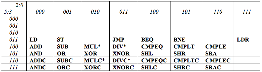 Although actual opcode assignments are generally uninteresting to the programmer and may be assigned arbitrarily, they are often grouped by instruction type or on some other logical basis. There may be implementation advantages to certain features of the assignments; for example, the fact that the functionally similar BEQ and BNE opcodes differ by a single bit may make it convenient to share the mechanism that interprets and executes them.

14.8.7.1. Unused Opcodes

Note that many of the possible 6-bit opcodes are unspecified in the table: they constitute unused opcodes (UUOs) whose function has not been specified in the ISA. The UUOs may be viewed as reserved for future expansion: subsequent versions of the Beta ISA might assign opcodes, for example, to floating-point operations or instructions for accessing individual bytes of main memory.

Alternatively, the UUOs may serve to allow some degree of implementation-specific customization of the instruction set. A manufacturer of signal-processing equipment might, for example, extend the Beta with application-specific instructions for a custom processor used in her products. Even users of off-the-shelf stock Beta processors may extend the instruction set by software (via mechanism to be discussed shortly).

While these alternative perspectives regarding UUOs -- and others -- are legitimate, there are tensions among them. To the extent that the ISA establishes a standard for the Beta, use of unspecified or functionally ambiguous aspects undermines the guarantee that software written to that ISA will run on hardware that implements the ISA. A user who writes software for a customised Beta ISA forgoes compatibility with existing Betas, although her software might run alongside existing software on an extended Beta. Two users building on mutually incompatibile ISA extensions guarantee that their software will never run on the same processor.

History has shown that careful thinking about major abstractions like the design of an ISA is a worthwhile engineering investment. An ISA that aspires to transcend several generations of hardware technology, for example, needs to provide an evolutionary path for the hardware/software interface. An ISA designed to support multiple implementations reflecting a variety of cost/performance tradeoffs might provide alternative implementation approaches to certain functions. For example, an ISA might specify floating-point instructions that are implemented in (slow) software in cheap CPUs and in (faster) hardware in higher-end processors. Each processor in this spectrum can execute the same software, albeit at varying speeds and cost.

14.8.7.2. Handling UUOs

Recognising that certain opcodes are unused in our ISA raises a subtle question: should the ISA specifiy the behavior of the Beta when it encounters an instruction containing one of these illegal opcodes? And if so, what behavior is desirable?

There are a number advantages to the careful handling of UUOs (and other error conditions that may arise) and the complete specification this handling in the ISA. A key capability is the ability for an error to invoke a software handler, whose execution somehow deals with the error. The handler might simply give a coherent error message. More ambitious handlers might perform a divide operation in software, masking the fact that the current Beta does not provide hardware support for the DIV instruction.

14.9. Exception Handling

Handling of UUOs motivates the remaining aspect of our ISA specification: dealing with various computational events that are extraneous to the normal steps in instruction execution. We use the term exceptions to describe this class of events, which fall into three categories:

• Faults represent error conditions that arise as a result of executing an instruction. Examples include illegal opcode errors arising from attempts to execute instructions having unimplemented opcodes, out-of-bounds-access faults resulting from access to a main memory location beyond the range of addresses available on the machine, or a divide-by-zero fault resulting from a division by a zero denominator.
• Traps are similar to faults, but are the intended consequence of instruction execution. For example, a UUO whose execution invokes a handler that emulates an unsupported hardware instruction may provide a measure of software compatibility at low cost.
• External Interupts are events generated by external stimuli, such as input/output devices. Examples include a keyboard interrupt that signals the fact that a key has been struck, or a network interrupt that signals the arrival of a packet of network traffic.

All three classes invoke the same exception handling mechanism, and we will see detailed examples of each in the third module of this course. For the present, we sketch the basic mechanism necessary to for their support.

14.9.1. Invoking a handler

The key mechanism required for processing exceptions is the ability to specify, for each exception type, a handler to be run when that exception occurs. A handler is simply a Beta program, stored as a sequence of Beta instructions in some region of main memory, whose execution is triggered by the computational event associated with the exception.

Each type of exception interrupts the execution of the currently running program, temporarily "borrowing" the CPU to run the handler code to deal with the exception. In the case of traps and external interrupts, the handler returns control to the interrupted program, which continues executing from the point at which it was interrupted.

The invocation of a handler simply requires loading the Beta's PC with the starting address of that handler, and executing instructions from there. However, there are several closely related characteristics we require from our mechanism for exception processing:

• Information preserving: The state of the interrupted program must be preserved (so it can be restarted), and accessible to the handler code (for error diagnosis or instruction set extension);
• Transparency: It must be possible to interrupt an arbitrary program, and return to that program without effecting its subsequent execution. The interrupt is thus invisible to the interrupted program.

We will place most of the burden of these requirements on the exception handlers themselves: they must be carefully coded to be information preserving and transparent. However, our minimalist architectural support cannot lose information in their invocation. Since invoking an exception handler necessarily involves loading its address into the PC, the prior contents of the PC -- critical state of the interrupted program -- will be lost unless we take steps to preserve it.

There are a variety of different approaches taken by contemporary CPUs to preserve the state of interrupted programs, including the PC. The approach taken by the beta simplifies its hardware complexity, at the cost of one register from its pool of 32:

1. One of the Beta's general registers, R30, is dedicated to use by exception processing. We memorialize this dedication by renaming it XP, for eXception Pointer.
2. XP is not to be used for ordinary programming, e.g.applications.
3. Each type of exception is assigned a unique address in main memory for an interrupt vector, a single Beta instruction that branches to the handler for that exception.
4. An exception of type $e$ is processed by the two step sequence:
   
   XP ← PC+4
   PC ←$IVector_e$
   
   where $IVector_e$ is the interrupt vector address assigned for exceptions of type $e$.
5. To maintatin transparency, interrupt handlers must save all CPU state (e.g. contents of registers) and restore it prior to returning to the interrupted program.
6. Since the value in XP is the address of the instruction following the interrupted instruction, a handler for an external interrupt will typically return to the interrupted program via a sequence like SUBC(XP, 4, XP) JMP(XP)

Beta interrupt vectors are assigned low memory locations, starting at zero. Location 0 is assigned to the RESET exception, which signals the startup of the CPU (e.g., on power-on). Location 4 is assigned to the IllOp exception, taken when an instruction containing an unused opcode is encountered. Other exception types, e.g. for I/O events, are assigned following locations.

14.9.2. Kernel Mode

In the Beta, interrupt handlers are part of the operating system kernel, a body of code permanently installed in a region of main memory that is a topic of the final module of this course.

Typically the operating system kernel is priviledged, in that it may directly access I/O devices and other basic system resources that unpriviledged programs, such as applications, access only via requests to the operating system. For this reason, it is common to maintain a bit of CPU state that distinguishes whether the CPU is currently executing priviledged OS code -- eg an interrupt handler -- or unpriviledged user code. In the Beta we dedicate the high-order bit -- bit 31 -- of the PC as the kernel mode bit: it contains 1 while executing code within the operating system kernel, or 0 while executing ordinary applications. We refer to these modes of CPU operation as kernel and user modes, respectively.

When a user mode program is interrupted by an exception, its PC (with a high-order 0 indicating user mode) is copied to XP, and the handler is entered with the kernel bit of the PC set to 1 ensuring that the handler runs in kernel mode. When the handler returns to the interrupted program via a JMP(XP) instruction, the entire PC -- including the K bit -- is restored from the value in XP. This restores the CPU to user mode to continue executing the program.

14.9.3. Reentrance

Although some systems allow the execution of exception handlers themselves to be interruped by exceptions, such reentrant handler execution presents some new difficulties. Since we have allocated the single register XP to hold the address of the interrupted program, for example, what happens if the handler is interrupted before it is able to save XP elsewhere? Such problems are solvable, but at some cost in complexity. As a result, handler reentrance is often avoided rather than being supported.

A simple way to avoid reentrant interrupts is to make the processor only take exceptions while in user mode. This requires that the operating system kernel be carefully written, both to avoid errors (which may not be properly handled) and to avoid depending on trapped instructions for functional extensions.

The Beta follows this route. Errors and traps are best avoided in kernel mode code, and attention to external interrupt requests from I/O devices is deferred until the CPU is running in user mode. This implies that the Beta will turn a deaf ear to I/O devices while in kernal mode, and must return occasionally to user mode to process external interrupt requests. The impact of these constraints on operating system structure will be explored in the next module of this course.

14.10. Factorial in Software

The Beta ISA introduced in later sections of this chapter provide minimalist but representative support for contenporary programming practices. Subsequent chapters will provide many substantive examples, illustrating typical software conventions for application and operating system programming.

  N:    (input value)

        ...

        // Compute Fact(N), leave in R0:
  Fact: ADDC(R31, 1, R0)  // R0 <- 1
        LD(R31, N, R1)    // load N into R1

  loop: MUL(R0, R1, R0)   // R0 = R0 * R1
        SUBC(R1, 1, R1)   // R1 = R1 - 1
        BNE(R1, loop, R31)// if R1 != 0, branch

        // HERE with R0 = Fact(N)
  

We close this chapter with a glimpse at a tiny fragment of assembly language code, shown to the right, that performs the same Fact(N) computation that we addressed with ad-hoc hardware in Section 14.1. Although details of the assembly language will be the subject of the next chapter, the astute reader will notice that the little program contains a sequence of five symbolic Beta instructions that have been discussed in this chapter, each on a separate line. The 32-bit binary translations of each symbolic instruction are stored in five consecutive locations in the Beta's main memory.

Comments in the code begin with // and extend to the end of the line, and are ignored by the translation to binary instructions. Notations like Fact: and loop: are tags that establish symbolic names for the memory address containing the following instructions; thus Fact denotes the memory address containing the first of the five instructions, and loop is the address of the subsequent MUL instruction. Another memory location, bearing the tag N:, is reserved to hold the input value $N$.

The instruction of the sequencer, ADDC, initializes R0 to 1 by computing the sum of zero (always the contents of R31) and the constant 1. The second loads R1 with the input value stored in the location tagged N:, via a load from the address computed by adding zero to the symbolic address N of the tagged location. These steps roughly correspond to the initializations performed in the start state of the FSM diagrammed in .

The remaining three instructions correspond to the looping state of that FSM, successively updating R0 by a new product while counting down the value in R1 until it reaches zero. The BNE(R1, loop, R31) is translated to an appropriate branch instruction whose constant portion is computed to make the target of the conditional branch be the instruction bearing the tag loop: -- the MUL instruction. In this case the constant computed will be -3, branching backwards three instructions from the location following the BNE. The branch to loop is taken whenever the value in R1 is nonzero; once R1 is counted down to zero, control will pass to the following instruction with the computed value left in R0.

14.11. References

• Beta ISA reference
• Single-sheet Beta summary, a useful cheat-sheet to have around when working Beta-related problems.

14.12. Further Reading

• von Neumann, John, First Draft Report on the EDVAC (1945). Incomplete draft by von Neumann detailing what became known as the von Neumann architecture.
• Hennessy, John L., and Patterson, David A., Computer Architecture: A Quantitative Approach, Fifth Edition, Elsevier 1012. Leading contemporary text on computer architecture, by the two best-known proponents of the RISC movement.
• Cohen, Danny, "On Holy Wars and a Plea for Peace", 1980.