
3. Information
This subject focuses on systems whose goal is the processing of information; that is, systems which take information as their inputs and produce information as their outputs. Much of its focus is on technology for representation of information and useful manipulations of these representations.Informally, information is knowledge. A common informal definition of information is "knowledge communicated or received concerning a particular fact or circumstance", suggesting the key role of information in communication (e.g., by sending and receiving messages). Moreover, the constraint "concerning a particular fact or circumstance" narrows the scope of the information considered in a message to some specific question or issue. If I'm interested in the outcome of yesterday's Red Sox/Yankees game, a note saying "The Sox Won" may be taken to convey that single-bit result regardless of whether its written in pen or pencil, the color of the paper, or the beer stain that decorates it. Our discussions of information and communication typically involve the abstraction of information, explicitly or implicitly, that is relevant to a particular question being answered.
A more subtle aspect of communication is that the information conveyed must be new to the receiver: if I tell you something you already know, I have communicated no knowledge and hence conveyed no information. If a message actually communicates something to the receiver, it must somehow increase the state of the receiver's knowledge; moreover, the amount of information conveyed is a measure of the amount by which the receiver's knowledge has increased. Informally, a message that contains a predictable fact conveys little information while one containing surprising news conveys more. The amount of information transferred by a message thus reflects not only the details of the message, but the initial state of the receiver as well.
3.1. Quantifying Information
These intuitive properties of information were formalized in 1948 by Claude Shannon. He modeled communication as a transmitter containing some information source connected to a receiver via a communication channel that conveys a stream of discrete symbols at the transmitter to a similar stream at the receiver. The channel can be viewed as an idealized communication and/or storage mechanism whose output stream is a replica of its input sequence, delayed in time and shifted in space. Shannon considered both noiseless channels, in which the output is a perfect replica of the input, and noisy channels in which the output may contain errors relative to the input.In this chapter we will assume that communication over a channel consists of messages, each encoded as a finite sequence of symbols, conveyed sequentially by the channel between the transmitter and the receiver. Following Shannon, we model the source of information as a random variable and the goal of the communication as the education of the receiver regarding the value of that random variable.
3.1.1. Information conveyed by a message
Using the insight that communication of information resolves uncertainty in the knowledge of the receiver, Shannon quantified the information conveyed by a message as a logarithmic measure of its predictability.More specifically, consider a discrete random variable $X$ having $N$ possible values $\{x_1, x_2, ..., x_N\}$ which occur with some known probabilities $\{p_1, p_2, ..., p_N\}$. Assuming this probability distribution is the only thing known about the value of $X$, a message that specifies $x_i$ as the value of $X$ conveys \begin{equation} I(x_i) = \log_2\left({1\over{p_i}}\right) \label{eq:info1} \end{equation} bits of information. Note that the use of inverse probabilities in this measure corresponds to our intuition that reporting probable facts conveys less information than reporting low-probability (surprising) ones. The logarithm in the formula gives the measure a satisfying additive property, and the choice of a logarithm base 2 leads to the conventional binary bit as our unit of information.
Examples:
- Suppose you're awaiting the result of the flip of a fair coin. In this case the possible values are $\{heads, tails\}$ with probabilities $\{0.5, 0.5\}$. Whichever result you learn, the gained information is ${\log_2}(1/0.5) = \log_2(2) = 1$ bit.
- A ball is drawn randomly from a hat containing 3 blue and 5 red balls, and you learn the color of the ball. Now the probabilities are $\{p_{red} = 5/8, p_{blue} = 3/8 \}$. The "ball is red" message conveys $\log_2(8/5) = 0.68$ bits of information, while a "ball is blue" message conveys $\log_2(8/3) = 1.4$ bits.
3.1.2. Partial resolution of uncertainty
Consider next the common case where the random variable $X$ takes on one of $N$ equally probable values $\{x_1, ..., x_N\}$ and that value is reported in a message. Since each such message occurs with probability $1 / N$, the information content in each message is $\log_2(N)$ bits by equation \eqref{eq:info1}. Note that, consistent with our intuition, our uncertainty regarding the choice of equally probable values increases with the number of possibilities; consequently, the information content of a message resolving that uncertainty increases as well.We can extend this example by considering messages that convey some information about the value of $X$, but leave some remaining uncertainty. In our case of finitely many equally probable values, we can model such partial resolution of uncertainty as a message $Z_{N>M}$ that decreases the number of equally probable values from its initial value of $N$ to some lower number $M$ of (again, equally probable) values. The information content of such a mesage is \begin{equation} I(Z_{N>M}) = \log_2\left({N\over{M}}\right) \label{eq:info2} \end{equation} After receipt of $Z_{N>M}$, the receiver is left with only $M$ possible choices for the value of $X$, hence less uncertainty. A subsequent message $Z_{M>1}$ that completely resolves the remaining uncertainty will carry $\log_2(M)$ bits of information (again by equation \eqref{eq:info1}). It is satisfying to observe that the total amount of information conveyed by the cascaded pair of messages $Z_{N>M}$ and $Z_{M>1}$ which together completely specify one of $N$ values is given by their sum \begin{equation} I(Z_{N>M>1}) = \log_2\left({N\over{M}}\right)+ \log_2\left(M\right) = \log_2\left({N\cdot{M}}\over{M}\right) = \log_2(N) \end{equation} and corresponds to the number of bits carried by a single message that specifies one of $N$ equally probable values in a single step. Equation \eqref{eq:info2} allows us to decompose information about an $N$-way choice into a sequence of messages successively narrowing the number of possibilities. Each such message conveys some amount of information to the receiver; when the cumulative total is $\log_2(N)$ bits -- all the information there is regarding the value of $X$ -- the receiver can determine the value of $X$ precisely.
Example:
-
Suppose Alice is trying to guess a randomly-selected single digit number $X$.
She learns the value of $X$ by a sequence of three messages, received in
the following order:
- Bob tells her that $X$ is less than 8.
- Charlie tells her that $X$ is odd.
- Don tells her that $X$ is divisible by 7.
- Charlie tells her that $X$ is odd.
- Don tells her that $X$ is divisible by 7.
- Bob tells her that $X$ is less than 8.
Since the information transferred by each message reflects Alice's apriori knowledge when she receives that message, the allocation of information among the messages may depend upon the order in which they are received. Suppose the order of the messages received by Alice was instead:
3.2. Encoding Messages
In the next Chapter, we will address the problem of representing individual bits as physical quantities that can be transmitted, stored, and manipulated reliably. For the remainder of this Chapter, we will assume that we are dealing with a binary channel capable of conveying a sequence of single-bit values from transmitter to receiver, and consider ways to use this channel efficiently.Our general formulation of this problem assumes that the transmitter is required to commuicate a sequence of messages to the receiver. Each such message is drawn from the set of messages $\{M_1, M_2, ..., M_N\}$, that occur with probabilities $\{p_1, p_2, ..., p_N\}$ respectively, where the probabilities in this set sum to 1. Our goal is to encode each message $M_i$ as a codeword $C_i$, consisting of a finite string of ones and zeros to be sent to the receiver via the channel. As we shall see, many alternative encoding strategies are possible, and they vary in the efficiency with which they use the channel. Our measure of efficiency of the encoding involves minimizing the number of bits that we require the channel to communicate, reflecting our assumption that there is some cost (in time, energy, or other parameter) associated with each bit transmitted.
3.2.1. Fixed-length encodings
The simplest encoding strategy for our $N$-messsage set is to assign a unique $k$-bit codeword to be transmitted for each of the $N$ messages. The uniqueness requires that the fixed codeword size $k \ge \log_2(N)$, and we generally choose the smallest $k$ that meets this constraint to avoid transmitting more bits than necessary.
| Message | Codeword |
|---|---|
| $M_i$ | $C_i$ |
| 0 | 0000 |
| 1 | 0001 |
| 2 | 0010 |
| 3 | 0011 |
| 4 | 0100 |
| 5 | 0101 |
| 6 | 0110 |
| 7 | 0111 |
| 8 | 1000 |
| 9 | 1001 |
Note further that this encoding uses only 10 of the 16 possible 4-bit codewords. This reflects the fact that each 4-bit codeword can carry 4 bits of information, while the information content of each decimal digit (assuming they're equally probable) is $\log_2(10) = 3.322$ bits. The difference between the 4-bit codeword and its 3.22-bit information content, as well as the unassigned codewords, reflect some inefficiency in our encoding: a fraction of the information-carrying capacity of our channel is being wasted.
Fixed-length codes are commonly used owing to their conceptual and implementation simplicity. The ubiquitous 7-bit ASCII standard represents English text by mapping each of about 86 charaters (upper- and lower-case letters, punctuation, digits, and math symbols) to a unique 7-bit code, conveying $\log_2(86) = 6.426$ bits of information in each 7-bit string.
3.2.1.1. Binary Integers
A particularly useful class of fixed-length encodings involves the representation of natural numbers -- non-negative integers -- as $k$-bit strings for some chosen size $k$. The codeword for each number $x$ corresponds to its natural representation $x_{k-1}x_{k-2} ... x_1x_0$ as a base 2 number, i.e. assigning a weight of $2^i$ to each bit $x_i$, so that the value $x$ becomes the weighted sum \begin{equation} x = \sum_{i=0}^{k-1}{2^i}\cdot{x_i} \label{eq:binary_number} \end{equation} Thus a $k$-bit string of 0's represents 0 while a $k$ bit string of 1's represents ${2^k}-1$, the maximal value representable as a $k$-bit binary number.
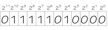
12-bit binary number
Since binary numbers are common currency in digital systems, we frequently need to cite them in programs and documentation (including these notes). For reasonable values of $k$, however, a $k$-bit binary representation is tediously long, while converting to and from our familiar decimal representation is tediously time-consuming. Consequently, the computer community often compromises via the use of hexadecimal (or base 16) representation of binary values, which are both concise and easy to convert to and from binary.
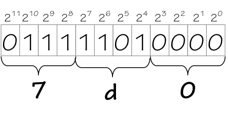
Binary to Hex Conversion

The correspondance between hex digits and 4-bit binary equivalents is summarized in the table to the left. Frequent users of hexadecimal quickly internalize this table, mentally mapping hex digits to binary implicitly as they are encountered. This can be a valuable skill when reasoning about arithmetic and logical operations on binary numbers that are represented in hex.
In order to distinguish between binary, decimal, and hexadecimal
representations, we often adopt a convention from the programming community
and use prefixes "0b" and "0x", respectively, to designate binary and
hexadecimal representations. Thus 0b011111010000 = 2000 = 0x7d0,
where the unadorned 2000 is presumed to be decimal.
3.2.1.2. Two's Complement Representation
There are a variety of approaches to the representation of signed integers as bit strings; of these, the two's complement representation has emerged as a de-facto standard. A $k$-bit two's complement representation of an integer $x$ is identical to the representation of $x$ as unsigned binary, with a single important exception: the weight of the high-order digit is negative ($-2^{k-1}$ rather than $2^{k-1}$). Thus the three-bit two's complement representation of 3 is $011$, while $101$ represents $-{2^2}+2^0 = -3$.This representation has several convenient properties:
- A negative number is easily distinguished by a 1 in its high-order bit position (often termed the sign bit).
- Each $k$-bit string represents a unique signed integer, in the range $-2^{k-1} ... 2^{k-1}-1$; and all signed integers in that range have a unique representation in $k$-bit two's complement.
- Arithmetic operations on two's complement integers are straightforward. For example, the addition of $k$-bit two's complement integers requires precisely the same mechanism as addition of $k$-bit unsigned binary integers: a single $k$-bit adder module can be used to deal with both representations.
- The unique representation of zero as a $k$-bit two's complement integer is a string of $k$ zeros. It follows from this and the prior properties that a string of $k$ ones represents -1 and that $A+\overline{A} = -1$ whence $-A = \overline{A} + 1$, where $\overline{A}$ represents the bitwise complement of $A$.
The price we pay for these advantages include several minor annoyances:
- Negating a $k$-bit two's complement integer is slightly tedious: in general, we complement each of the $k$ bits (changing 0 to 1 and 1 to 0), and then add 1 to the $k$-bit result.
- An assymmetry in the range of positive vs. negative integers that can be represented: a $k$-bit two's complement number can represent one number -- $-2^{k-1}$ -- whose negative $2^{k-1}$ cannot be represented using $k$-bit two's complement. This stems from the fact that the total number of $k$-bit representations $2^k$ is even, and we require a unique representation for zero; thus an odd number of representations are left to be allocated to positive and negative numbers.
3.2.1.3. Representation of Real Numbers
Extending our representation of numbers beyond integers typically involves some convention for representing approximate values of real numbers over some specified range, using finite ($k$-bit) strings. One simple approach is to combine $k$-bit two's complement representations with a constant scale factor that is agreed upon as part of the representation convention. To represent the dollar price of products, for example, we might choose a scale factor of $1/100$, whence the string $011111010000$ indicates a $\$$20.00 price rather than the $\$$2000 it would signify if interpreted as unscaled binary. Such conventions amount to the use of integer representations together with smaller units -- in this case, using pennies rather than dollars as our unit of currency.Such scaled binary representations often choose a negative power of two as the scale factor, which has the effect of moving an effective "binary point" from its implicit position to the right of the low-order bit position. Thus a 12-bit two's complement representation with a scale factor of $2^{-6} = {1 / 64}$ reinterprets our binary $011111010000_2 = 2000_{10}$ as the scaled binary $011111.010000_2 = 31.25$.
Representation of approximate real numbers over a wider dynamic range commonly involves floating point representations, in which a number $x = f\cdot{2^e}$ is represented by a pair of twos-complement integers specifying values for the fraction $f$ and exponent $e$ respectively. Floating point representations are commonly supported in hardware in modern processors, and have been highly optimized using a number of representation tricks.
3.2.1.4. Limits on Numeric Representations
The conventions discussed so far for represention of numbers presumes that each number is represented by a $k$-bit string, for some finite constant $k$. Each such convention necessarily constrains the universe of representable values to at most $2^k$ distinct values, the number of available representations; this limits the range of representable integer data, as well as the precision with which real numbers are approximated using floating point conventions. Because the fixed-size assumption greatly simplifies the implementation technology, fixed-size representations are most commonly used.It is possible to relax these constraints by allowing the representation of each number to expand to an arbitrary (finite) number of bits. One example of this approach uses variable-sized bit strings to precisely represent integers of arbitrary size, limited only by the size of availble storage. Such representations (often termed bignums or arbitrary-precision integers) are useful in certain applications, and commonly supported by software libraries managing their implementation as data structures. Since pairs of bignums can be used to precisely represent arbitrary ratios $m/n$ of integers, arbitrary-precision arithmetic can be extended to include precise representations of rationals as well as integers.
None of these encoding conventions are capable of exactly representing arbitrary real numbers; at best, they deal with rational approximations. It is sometimes mistakenly assumed that computers are incapable of precisly representing an irrational real value like $\pi=3.14159...$, as any encoding would require infinitely many bits. In fact, we might easily adopt a convention, say, by which the two's-complement representation of each integer $j$ precisely represents $j\cdot\pi$; this convention allows $k$-bit quantities to precisely represent a universe of $2^k$ real numbers, all but one of which is irrational. Alternatively, we might adopt a convention for representing symbolic formulae in which the symbol $\pi$, or the ASCII string "Pi", precisely represents the value of Pi.
The lesson from the above example is that the fundamental constraint on our representation scheme is on the size of the universe of values represented, rather than on the values themselves. Using a $k$-bit fixed-size representation, we're limited to a finite universe of $2^k$ values. If we relax the fixed-size limitation (and ignore global limits on the number of bits available), the number of available encodings becomes the number of finite strings of ones and zeros. This set is countably infinite (meaning that there are as many such strings as there are integers), allowing systematic representation of integers and rationals (each of which is also countably infinite). But the set of real numbers is uncountably infinite: there are far more real numbers than finite bit strings. At best, we can represent countable subsets of the reals such as rational approximations or integral multiples of $\pi$.
3.2.2. Variable-length encodings
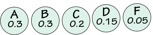
Because fixed-length encodings assign codewords of the same length to be transmitted for each message, they do not necessarily make efficient use of our communication channel. Suppose, for example, we are transmitting letter grades from the set $\{A, B, C, D, F\}$, each message conveying a single grade. Assume further that the probability with which each grade occurs is given by $\{p_A={0.3}, p_B={0.3}, p_C={0.2}, p_D={0.15}, p_F={0.05}\}$. A fixed-length encoding would assign a unique 3-bit string to each grade; thus transmitting, say, 1000 grades would require sending 3000 bits over the channel. We might ask whether a more sophisticated encoding scheme would reduce the channel traffic, and consequently the cost of transmission.3.2.2.1. Information Entropy
To evaluate the efficiency of our coding scheme, it is useful to calculate the expected information content of each symbol transmitted -- i.e., the average information per symbol over a large number of transmitted symbols. This measure, termed information entropy, reflects the actual information that we need to transfer per symbol, irrespective of the encoding we choose. It represents a lower-bound on the bits/symbol over all possible encodings: any scheme transmitting fewer bits per symbol must not be communicating all of the information available.To evaluate the information entropy of our current encoding problem, it is useful to summarize the symbols and their information content in a table as follows:
| Symbol S | Probabity $P_S$ | Information $\log_2(1/P_S)$ |
Weighted info ${P_S}\cdot{Info_S}$ |
|---|---|---|---|
| $A$ | 0.3 | 1.737 | 0.521 |
| $B$ | 0.3 | 1.737 | 0.521 |
| $C$ | 0.2 | 2.32 | 0.464 |
| $D$ | 0.15 | 2.737 | 0.41 |
| $F$ | 0.05 | 4.32 | 0.216 |
| Totals | 1.0 | 2.132 |
Given a fixed-length encoding that requires 3 bits per symbol transmitted versus an average information content of 2.132 bits per symbol, we conclude that the difference (0.868 bits/symbol) represents wastage of our channel capacity by a less than perfectly efficient encoding. We might seek to improve this efficiency via a more sophisticated coding technique.
3.2.2.2. Huffman Codes
One inefficency of our fixed-length coding is that it uses the same 3-bit codeword length for messages with low information content (like $A$) as is used for high-information messages (such as $F$). While a 3-bit codeword for $F$ seems a bargain -- conveying 4.32 bits of information in a 3-bit transmission -- this advantage is more than offset by higher-frequency messages like $A$ and $B$ which devote 3-bit codewords to less than 2 bits of actual information transfer. A general principle we can exploit to improve efficiency is to devote channel capacity (in this case, codeword bits) in rough proportion to the information content of each message. We see homey examples of this principle in everyday communications: a surprising (i.e., high-information) news item earns larger-type headlines than that devoted to routine articles, using a greater fraction of the communication resource (newspaper area) as a result.We can improve our channel usage efficiency by allocating longer codewords to messages carrying more information. Of course, we need to ensure (a) that each message is unique and (b) that the receiver can parse the stream of bits it receives into individual messages -- i.e., that it can recognise message boundaries. A nifty scheme proposed in 1951 by David Huffman provides a simple solution that remains commonly used today. Construction of a Huffman code involves building a graph whose nodes represent symbols -- or combinations of symbols -- to be transmitted to the receiver.
- Select two unparented nodes from the graph having the lowest probabilities.
To resolve ties resulting from identical probabilities, choose arbitrarily.
The first such selection in our example would be nodes for $D$ and $F$.
- Add a new node to the graph that becomes the parent of the two selected
low-probability nodes. Mark this node with the union of the symbols
appearing in the selected nodes, and with the sum of the selected
nodes' probabilities.
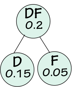
In our example, the first parent node would be $DF$ with a probability of $0.2$.
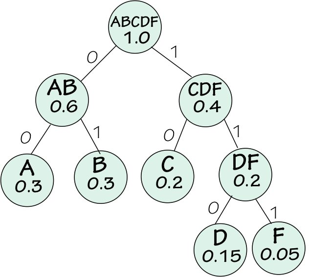
Huffman Coding Tree - Repeat steps 1 and 2 until all nodes are parented except for one root
node, listing all symbols and having probability of 1.
A graph like that shown to the right would result from our example.
- Finally, label edges of the two children of each parent node "0" and "1", assigned arbitrarily to the two edges.
DF Subtree
Our example Huffman code is summarized in the table below.
| Symbol S |
Probabity $P_S$ |
Codeword | Weighted info ${P_S}\cdot{bits}$ |
|---|---|---|---|
| $A$ | 0.3 | 00 | 0.6 |
| $B$ | 0.3 | 01 | 0.6 |
| $C$ | 0.2 | 10 | 0.4 |
| $D$ | 0.15 | 110 | 0.45 |
| $F$ | 0.05 | 111 | 0.15 |
| Totals | 1.0 | 2.2 |
Huffman coding provides optimally efficient use of our channel, so long as we insist on sending an assigned, separate codeword (containing an integral number of bits) for each symbol transmitted. We can do better, however, by encoding larger blocks of data -- sequences of symbols -- into composite codewords. These more sophisticated coding techniques can get arbitrarily close to the efficiency limit dictated by our entropy measure.
3.3. Data Compression
One familiar application for sophisticated encoding techniques is lossless data compression, the application of an algorithm to a file containing a finite sequence of bits to yield a shorter file containing the same information.
Each lossless compression scheme operates by discovering redundancy -- predictable structure in the supplied input -- and using some encoding trick to exploit that structure in fewer bits. For example, a run-length code might replace a sequence of 1000 consecutive ones with a short code containing the integer 1000 and the repeated value 1. Typical compression programs have a library of techniques to exploit such structure (and much more subtle redundancies as well).
3.3.1. Does recompression work?
Since a compression algorithm reduces one string of bits to another (shorter) string, one might be tempted to assume that compressing a compressed file shortens it even further. Suppose, for example, we start with a 6MB file containing the ASCII text of the King James Bible, and compress it using (say) zip. The result would be a shorter file -- perhaps 1MB. Would compressing that lead to a 300KB file? Can we continue until we have reduced the entire text to a single bit?The answer, of course, is no. Since lossless compression is reversible, repeated compression of a 6MB Bible down to a single-bit string would imply that repeated decompression of a single-bit string would eventually regenerate the original Bible text -- an implausible outcome, unless the original text were somehow embedded in the decompression program itself. In general, a compressed file has higher entropy (less redundancy) than the original file. If the compression works well, the resulting file has little remaining redundancy: its bits look completely random, exhibiting no predictable structure to be exploited by further compression. The original file has some intrinsic information content, and cannot be compressed beyond this point.
3.3.2. Kolmogorov Complexity
An appealing measure of the intrinsic information content of a string $S$ is the size of the smallest program that generates $S$ with no input data. This measure, termed Kolmogorov complexity (after the mathematician Andrey Kolmogorov), corresponds intuitively to the compressability of the string by lossless algorithms, and is a useful conceptual and theoretical tool.However, Kolmogorov complexity has two serious limitations as a practical measure of information content. The first of these is its uncomputability: there is no algorithm $K(S)$ which computes the Kolmogorov complexity of an arbitrary string $S$.
The second limitation is the dependence of Kolmogorov complexity on the language chosen for the programs considered. Given a particular string $S$, for example, the smallest Python program generating $S$ will likely be a different size than the smallest Java program, leading to different values for the Kolmogorov complexity of $S$. The impact of the language choice on Kolmogorov complexity is at most an additive constant: given programming languages $L_1$ and $L_2$, that constant -- the disparity between Kolmogorov complexities assigned for a string using the two languages -- is about the size of a program capable of translating programs from $L_1$ to $L_2$ or vice versa.
However, given the string $S$ and a program $P$ that generates $S$, one can construct an ad-hoc language $L_S$ such that the 1-character program "X" generates $S$, and any program whose first character is "Y" is interpreted by stripping the first character and processing the remainder in the language of $P$. Relative to this language, the Kolmogorov complexity of $S$ is 1, while that of other strings is one more than their complexity relative to the language of $P$. This leads to the awkward observation that the Kolmogorov complexity of any string is 1 given the right language choice. Such artificial constructions can be ruled out by agreeing on a particular language (such as that of a Universal Turing machine described in Chapter 13Chapter 13); however, there is no compelling argument for the choice of a "natural" language for this measure.
3.3.3. Lossy compression
The compression schemes discussed above are lossless in the sense that the compression process is perfectly reversible -- i.e., decompression of a compressed file yields a file identical to the original. No information is lost in a compression/decompression cycle.In many applications, alternative compression schemes are commonly used that reduce file size without guaranteeing that the original file is precisely recoverable. The algorithms used are specifically designed for a particular type of data, e.g. video streams, audio streams, or images, and incorporate some data-specific model about aspects of the medium where information content can be compromised (or approximated) at the cost of nearly imperceptable degradation of the end result. In general, lossy compression involves tradeoffs between perceived quality and amount of information; for example, compromising the resolution of certain details in a photo reduces file size.
Examples of commonly used lossy compression schemes include JPEG images, MP3 audio files, as well as coding schemes used in CDs, DVDs, and streaming services like Netflix and Amazon.
3.4. Communication over Noisy Channels
We next consider more realistic communication and storage models in which the channel connecting transmitter and receiver may distort the stream of bits conveyed. Real-world information channels are subject to noise and other sources of error; we model these here by a noisy channel that occasionally reports a transmitted 0 bit as a 1 (or vice versa) to the receiver.Although our encodings have thus far been designed to minimize redundancy in the transmitted codewords, in the following sections we will get a glimpse of techniques for introducing codeword redundancy to improve reliability of communication over noisy channels.
For illustration, we will assume a simple scenario in which the transmitter has a stream of single-bit symbols from the set $\{0, 1\}$ to be conveyed to the receiver via a noisy channel which also conveys streams of $\{0, 1\}$ bits with occasional flipped bits. The most straightforward "encoding" is to just send the transmitter's symbols directly over the channel: each $0$ at the source transmits the codeword $0$, and each $1$ transmits $1$. Unfortunately, errors introduced by the channel cause the receiver to get wrong data, with no notice that a problem has occured. Depending on the application, this may have disasterous consequences.
3.4.1. Single-bit error detection
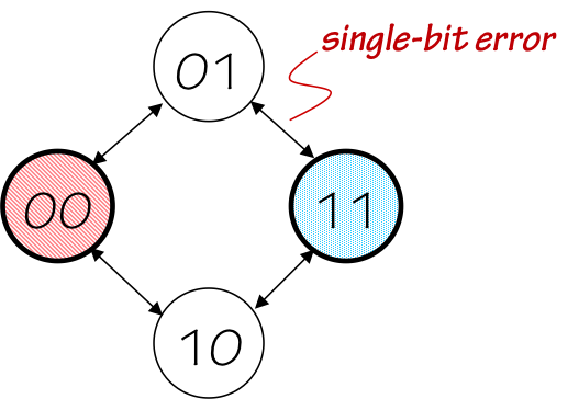
Suppose single-bit errors -- changing a 1 to a 0 or a 0 to a 1 -- happen infrequently and in isolation (rather than in bursts). It can be useful in such cases to consider encoding schemes that can reliably detect a single flipped bit in the context of a longer transmitted codeword. We can easily make isolated single-bit errors detectable by the receiver by the brute-force introduction of redundancy in our coding: simply transmit each bit twice! That is, transmit the codeword $00$ for each symbol $0$, and the codeword $11$ for each $1$. A single-bit error in either transmitted codeword will result in a received codeword of $01$ or $10$, each of which can be recognised as an error since neither will be sent by the transmitter.3.4.2. Hamming Distance
In cases involving only flipped-bit errors (as opposed to omission and/or insertion of error bits), a useful measure of the distortion inflicted on a codeword $C$ is the number of bit positions that differ between the transmitted $C_T$ and the distorted (but same length) replica $C_R$ seen by the receiver. We call this number the Hamming Distance between $C_T$ and $C_R$; more generally, the Hamming Distance betweeen two equal-length strings is the number of positions in which the strings differ.
2-bit Codewords
The factor of two cost in channel usage of our bit-doubling scheme is high, but the one redundant bit we've added may be used to detect single-bit errors in arbitrarily large codewords. If we have an existing encoding with $k$-bit codewords, we can add a single parity bit to each codeword yielding an encoding with $k+1$-bit codewords and single-bit error detection. The transmitter may, for example, always transmit a value for the parity bit that makes the total number of 1s in the codeword odd (odd parity); if the receiver gets a codeword with an even number of 1 bits, it will signal an error. This commonly used technique uses a single parity bit to ensure valid codewords have a Hamming distance of at least two.
While a Hamming distance of 2 allows single-bit error detection, 2 or more errors may still go undetected. The addition of codeword bits to increase the minimum Hamming distance between valid codewords can allow the detection of multiple-bit errors in a codeword. In general, a minimum Hamming distance of $D+1$ is required to detect $D$-bit errors within a codeword.
3.4.3. Error Correction
Further increasing the Hamming distance between valid codewords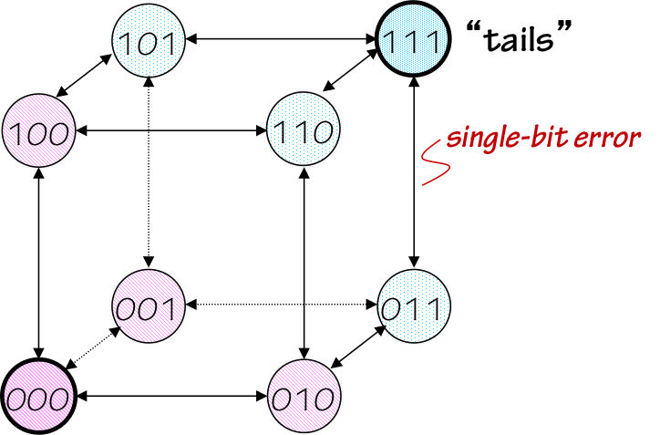
3-bit Codewords
More generally, we can correct $k$-bit errors by ensuring a Hamming distance of at least $2\cdot{k}+1$ between valid codewords. This constraint assures that a $k$-bit error will produce a mangled result which remains closest to the valid codeword that was actually transmitted.
3.5. Channel Capacity
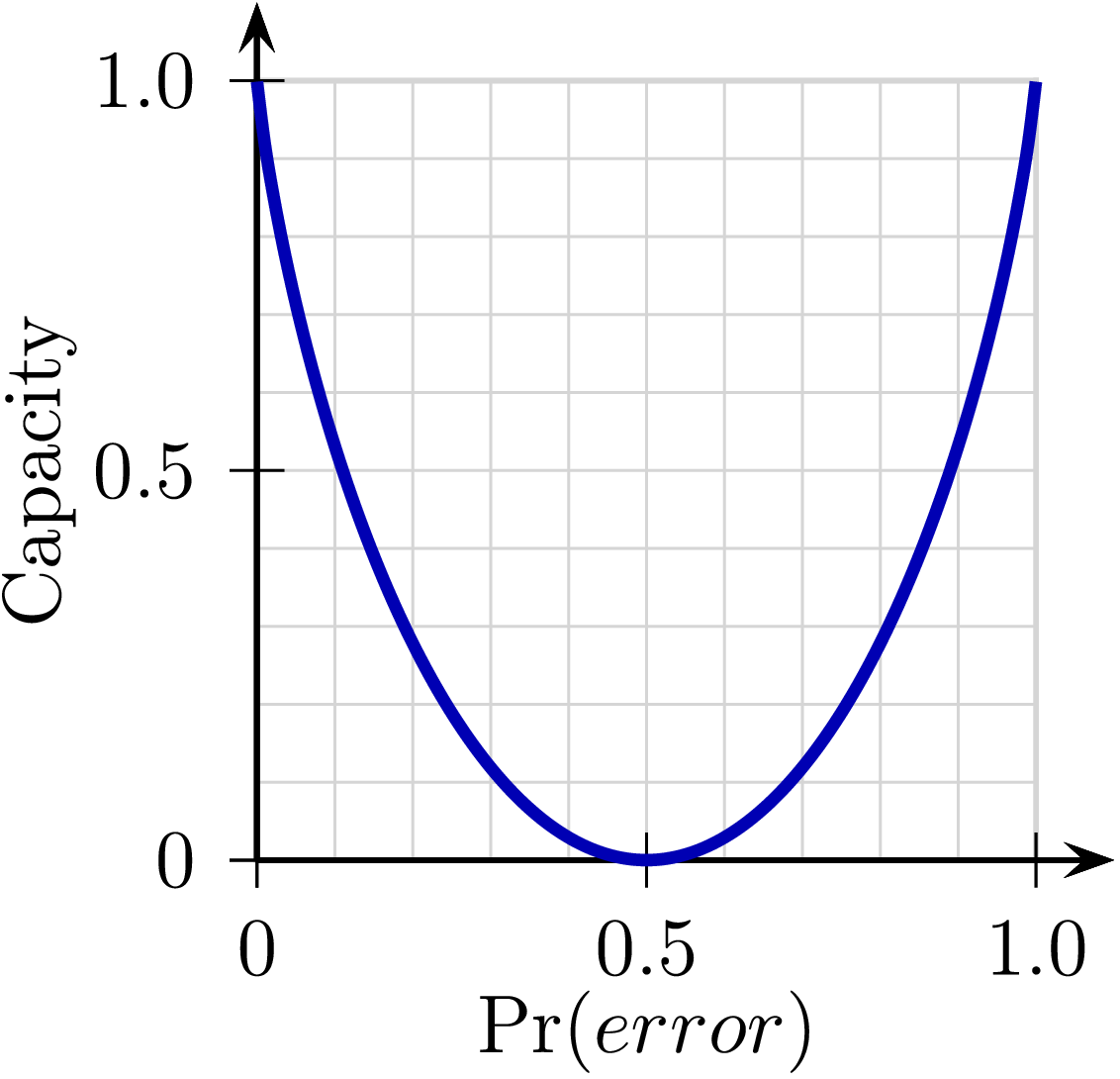
One might expect from our examples that a channel becomes fairly useless as error probabilities increase beyond some miniscule value, as the cost (redundancy) necessary to correct them exhausts the channel's communication capacity. In fact, that intuition is pessimistic. Shannon showed that any channel whose output is not completely independent of its input can be used for reliable communication via appropriate encoding techniques.The noise properties of of a channel -- e.g., the fraction of bits that are flipped in the simple binary channels we have considered here -- dictate a channel capacity $C$ for that channel, an upper bound on its rate of reliable information flow. It is impossible to communicate over the channel at rates greater than C, but, remarkably, sophisticated encodings can establish reliable communication at rates arbitrarily close to this capacity. Efficient encodings would involve error correction over large blocks of data, likely introducing significant delays between transmitter and receiver; but rates arbitrarily close to $C$ are possible.
Channel Capacity
The simple flipped-bit noise model considered here, called a binary symmetric channel, ignores possible complications such as error bursts, omissions, and insertions of noise bits. More sophisticated models consider these and other issues, leading to encodings that support reliable communication despite a wide variety of channel distortions.
3.6. Chapter Summary
Information is the principal commodity that is manipulated by the digital systems dealt with in this subject, and is quantified by its ability to resolve uncertainty. Important properties of information include:- A message that reduces $N$ equally-probable choices down to $M \lt N$ conveys $\log_2(N/M)$ bits of information.
- A message that identifies an outcome $i$ having probability $p_i$ conveys $\log_2(1/p_i)$A bits of information.
- The average information per message in a stream of symbols or entropy is $\sum p_i \cdot \log_2(1/p_i)$ where $p_i$ is the probability of the $i^{th}$ symbol in the alphabet used.
- redundancy reduces average information content per transmitted bit; efficiency of information storage or communication is thus enhanced by reducing redundancy through data compression.
- redundancy can, however, increase robustness by allowing
certain errors to be detected and/or corrected:
- Simple detection/correction codings intersperse invalid codewords, reflecting $k$-bit errors, between valid codewords actually transmitted.
- To detect $k$-bit errors requires an encoding whose valid codewords have a minimum Hamming distance greater than $k$;
- To correct $k$-bit errors requires an encoding whose valid codewords have a minimum Hamming distance greater than $2\cdot k$.
3.7. Further Reading
- Shannon, C., "A Mathematical Theory of Communication", BSTJ July 1948. Landmark paper introducing information, bits, entropy, and channel capacity.