Finite State Machines
9. Finite State Machines
The memory devices introduced in
Chapter 8 allow us
to build digital systems, and components of digital systems, whose
output reflects values of stored
state variables as well as current
inputs.
 Finite State Machine
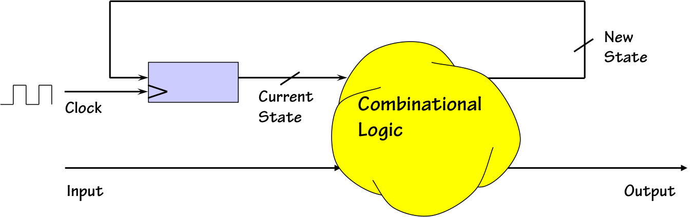
A common implementation for such systems, suggested in that chapter,
is sketched to the right. Its two major subsystems are a storage device
containing a digital representation of the system state, combined with
combinational logic that computes new values for state variables as well
as system outputs from the combined system inputs and current state
variable values.
This implementation approach is termed a
Finite State Machine
(
FSM),
a widely studied and commonly used abstraction for an important class
of sequential logic systems.
In this chapter, we explore the FSM both as an engineering abstraction
and as an important tool in our repertoire of digital engineering tools.
FSMs are a convenient model for certain classes of sequential systems,
typically those involving a modest number of discrete system
states
each of which is identified with some meaningful problem-related
circumstance.
We introduce the FSM abstraction by means of a simple example.
Example 1: Digital Combination Lock
9.1. Example 1: Digital Combination Lock
 Digital Combination Lock
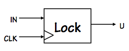
Consider a simple clocked circuit that serves as a primitive digital combination
lock. In addition to a clock, it takes a single input bit during each clock cycle,
and its output is an "unlock" signal whose value is to be 1 if and only if the
bits entered during the last four clock cycles corresponds to the secret four-bit
combination $0110$.
 Simple lock implementation
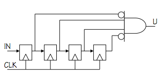
There are many approaches to designing such a circuit, one of which is sketched
to the left. This circuit simply stores the most recent four bits in four
flipflops, and generates its output via an AND gate with two inverted inputs
to recognize when the stored 4-bit value is $0110$.
While this is a reasonable implementation strategy for our lock, we might ask whether
a simpler implementation is plausible; in particular, whether $N$ flip flops are
needed for a lock having an $N$-bit combination.
To explore such issues, it is useful to describe the desired behavior of
the device in terms that are more detailed than its English description but
more abstract than a circuit diagram.
FSMs: The Abstraction
9.2. FSMs: The Abstraction
A finite state machine is a device which has
- A finite number $k$ of discrete states, $\{S_1, ..., S_k\}$,
one of which is designated as the initial state $S_i$;
- A finite number $m$ of digital inputs $\{I_1, ..., I_m\}$;
- A finite number $n$ of digital outputs $\{O_1, ..., O_n\}$;
- A set of transition rules specifying a next
state $s'(s, I_1, ..., I_m)$ for each state $s$ and set of inputs $I_1, ..., I_m$;
- A set of output rules specifying output values $O_1(s, I_1,...,I_m), ..., O_n(s, I_1,...,I_m)$
for each state $s$ and set of inputs $I_1, ..., I_m$
An FSM begins operation (e.g., on power-up) in its initial state.
At each active clock edge, it makes a
state transition
to a new state $s'(s, I_1, ..., I_m)$ dictated by the current
state $s$ and the current inputs $I_1, ..., I_m$.
The output values are dictated by the current state $s$, and
(optionally) the current inputs.
State Transition Diagrams
9.2.1. State Transition Diagrams
It is common to represent the behavior of an FSM as a graph whose
nodes represent states and whose edges represent transitions between
states.
Such a graph is called a
state transition diagram.
 FSM States
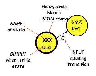
One notational convention is illustrated in the diagram to the right,
which shows a transition between a pair of states. The leftmost state
is distinguished as the initial state by a heavy circle. Each of the
two states are labeled with a name (an unimaginative $XXX$ and $XYZ$,
respectively), and (optionally) a value for the output when the FSM is
in that state.
The transition is shown by a directed edge from state $XXX$ to state
$XYZ$, labeled by the set of inputs causing this transition to be made.
Moore vs Mealy Machines
9.2.2. Moore vs Mealy Machines
There are two distinct variations of the FSM abstraction which
impact the state transition diagram notation.
Although the FSM definition in
Section 9.2
allows an FSM output to depend on both the current state $s$ and current input
values $I_1, ..., I_m$, output values are often constrained to reflect only
the current state and not the input values.
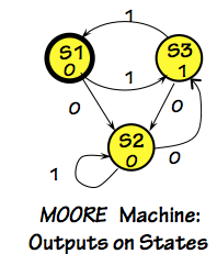
An FSM conforming to this restriction is called a
Moore machine.
The state transition diagram for a Moore machine typically labels
nodes (states) with output values, and transitions with input combinations
as shown to the right.
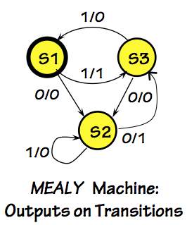
An FSM whose output reflects both current state and current inputs is termed
a
Mealy machine, and requires slightly different set of conventions
for its state transition diagram.
As Mealy machine outputs are not functions only of states, the edges of
a Mealy machine diagram are often annotated with output values as well
as input criteria, as shown on the left.
Note that, unlike most of our clocked devices, a Mealy machine may have
combinational paths between input and output terminals.
Such paths complicate the use of Mealy machines as components, since
combinational logic connecting an input to an output may introduce
a forbidden combinational cycle.
Although Moore and Mealy machines are both commonly used in practice, we
focus our attention here on the simpler Moore machine formulation for our
examples.
FSM Specification
9.2.3. FSM Specification
At the FSM abstraction level, the behavior of a machine can be specified
by a state transition diagram which is
complete in the sense
that it specifies unambiguous transitions and outputs for every current state/input
combination.
To satisfy this requirement, transitions leaving each state must be both
mutually exclusive and
collectively exhaustive, implying
that exactly one transition is specified for each state/input combination.
Returning to the example of a primitive 4-bit digital combination lock,
we can consider an FSM implemplementation in which each state implicitly
reflects the portion of the $0110$ combination entered thus far,
 Digital Lock FSM
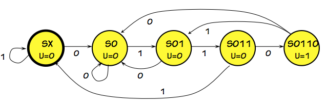
resulting in the 5-state FSM diagrammed to the right.
The initial state of this machine, $SX$, corresponds to the "power on" state:
no bits of the combination have as yet been entered.
If a $1$ is entered in the $SX$ state, we remain in that state (since
the first bit of the combination is $0$, no bits have as yet been entered).
If a $0$ is entered while in the $SX$ state, we transition to the $S0$
state to reflect that the first bit -- $0$ -- of the combination has
been entered correctly.
As successive bits of the $0110$ combination are entered, we progress
through states $S01$ and $S011$ to the state $S0110$ which specifies
a $U=1$ (unlock) output.
At any point along this path, an incorrect input bit causes the FSM
to transition to the state that properly reflects the number of correct
input bits entered thus far.
FSM implementation
9.2.4. FSM implementation
A given state transition diagram can be easily converted to a
hardware design that implements the FSM whose behavior it describes.
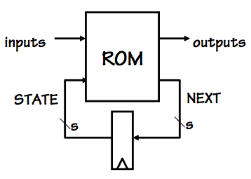 ROM-based FSM
Our strategy is to encode each of the $k$ states as distinct values
of a set of $s$
state bits, stored in an $s$-bit register
as shown in the diagram to the right.
Additional combinational logic -- e.g. a ROM as shown in this diagram --
is used to compute next state and output values as specified by the
FSM's transition diagram.
Given the five states shown in the state transition diagram for our
4-bit combination lock, it is clear that the minimum number $s$ of state
bits needed for this FSM is 3 (the smallest $s$ such that $2^s \ge 5$).
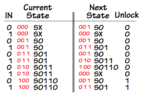 State Assignments
In translating a state transition diagram to a logic implementation,
it is convenient to rewrite the information it contains as a table
such as that shown on the left, first using symbolic names for the
states and then adding the assignment of unique values for the $s$
state variables.
Once assigned state variable values are supplied, the table becomes
a truth table for the combinational logic (e.g., ROM) of the FSM.
The state assignment -- mapping of discrete states to unique $s$-bit
strings -- may be completely arbitrary, as it is in this example.
However, it is often the case that a clever encoding of state
variables can simplify the FSM logic; for example, some of the
state variables may be used as outputs as well as recording internal
state.
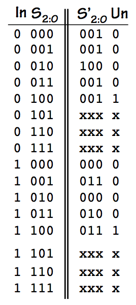 Lock ROM TT
Given the state assignments, it is straightforward to rewrite
the tabulated input and output combinations to produce a truth
table for a ROM or other combinational logic to complete the FSM;
a truth table for our primitive 4-bit lock is shown to the right.
Note that the truth table is incomplete, in that it contains
don't care values shown as $x$ in the output columns of
the table.
These values represent unused portions of the ROM: assuming we
arrange to start the FSM in the initial state $S_2S_1S_0=000$,
the $x$ values appear only for $S_2S_1S_0$ combinations that
represent
unreachable states in our implementation.
This wasted ROM space reflects the fact that we need to use
3 state bits, which could represent as many as 8 states,
for a 5-state machine.
As our lock FSM is a Moore machine, the output
Unlock
bit reflects only the current state: it is $1$ if and only if
$S_2S_1S_0=100$.
In a Mealy machine, this constraint would not apply.
States versus Bits
9.2.5. States versus Bits
It is interesting to note that the implementation of our 5-state
FSM requires only 3 flip flops, in contrast to the 4-bit shift
register implementation shown in
Section 9.1.
If we generalize both implementation strategies to locks having $N$-bit
combinations, we notice that the earlier strategy requires $N$ bits
of storage, while the latter requires $N+1$ states and hence about
$log_2(N)+1$ bits.
For our 4-bit lock this difference is not dramatic, but it is
important to recognize the exponential cost difference between
these approaches as $N$ becomes large.
More generally, we can think about systems with storage in terms
of
bits stored or
states, and these alternative
views are exponentially related (since $k$ bits of storage exhibit
$2^k$ distinct states).
Each view is useful in certain circumstances.
Asynchronous Inputs
9.2.6. Asynchronous Inputs
Our primitive lock is a clocked sequential device, whose reliable
operation requires that its inputs obey the dynamic discipline:
they must obey setup and hold times dictated by our implementation.
This constraint is manageable so long as the inputs are generated
by another sequential device sharing the same clock as our FSM,
the common case when we are constructing large sequential systems
from clocked components.
In the case of a combination lock, however, we might reasonably
require that the input bits are coming from a human pressing buttons
rather than a clocked machine.
We can't assume that the human is aware of the details of our FSM's
clock timing, or the setup and hold times required by our device.
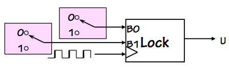 Two-button lock FSM
We might construct a more practical version of our lock
using two input buttons $B_0$ and $B_1$ as shown on the
right, allowing the user to press $B_0$ to enter a $0$
or $B_1$ to enter a $1$ as the next bit of the combination.
Each of the inputs has the value $1$ only when the corresponding
button is pressed; we assume that the clock is fast compared to the frequency
of button presses, so that many clock cycles will go by for each
consecutive bit entered by a button press.
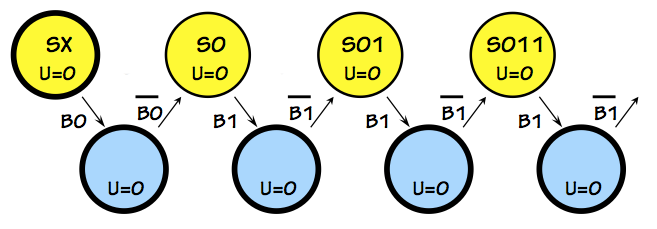 Added wait states
We can accommodate these extra clock cycles in our FSM by adding some additional
FSM
wait states to our FSM, as sketched to the left.
Each of the added states is entered when a button is pressed, and is left only
when that button is subsequently released (many clock cycles later).
The observant reader will note that while this approach deals with the
disparity between the rate at which a human enters input bits and the frequency
of our clock, the input changes on $B_0$ and $B_1$ remain asynchronous
with respect to the clock.
Thus we cannot guarantee that any setup and hold time restrictions we
place on the timing of these inputs will be met by our unsynchronized
(human) source of input values.
This important remaining problem is the subject of
Chapter 10.
FSM Properties
9.3. FSM Properties
The characterization of FSMs by their number of states, rather
than their total amount of storage in bits, leads to a geometric
increase in their size (in terms of states) as small FSMs are
combined to make bigger ones.
We have seen that an FSM implemented using $k$ bits of storage
as shown to the left has at most $2^k$ states; hence adding a single bit
of storage potentially doubles the number of states.
 m*n-state FSM
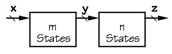
Moreover, an FSM constucted using an $m$- and $n$-state FSMs as components
may have as many as $m \cdot n$ states, as each state of the combined FSM
corresponds to a pair of states from the component FSMs.
This corresponds to our intuition regarding their implementation, as
the total storage required for the combined machine is about $log_2(m)+log_2(n) = log_2(m \cdot n)$.
FSM Party Games
9.3.1. FSM Party Games
 Mystery FSM
Consider a geek party game in which you are handed an unknown FSM like the one shown to the left
and asked to discover its behavior (i.e., to figure out its state transition diagram).
The mystery FSM has two buttons labeled $0$ and $1$, and makes a transition on each button press.
Its single output is a light which is on in some states and off in others.
It also has an on/off switch which can be used to return the FSM to its initial state.
Can you discover the behavior of this FSM without disassembling it?
In general, you cannot reverse-engineer the black-box FSM in finitely
many experiments, unless you are given some upper bound on the number
of its states.
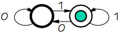
Suppose, for example, you spend a few minutes trying input sequences,
and notice that the light goes ON each time you press the $1$ button
and OFF each time you press $0$.
You might reasonably conclude that the FSM is the simple 2-state machine diagramed to the right,
based on your experiments: its a straightforward ON/OFF switch.
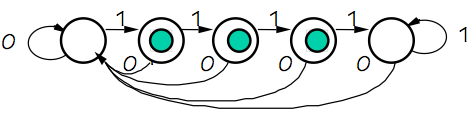
Such a conclusion is premature, however;
there are some input sequences not represented in your experiments.
Your host might demonstrate, for example, that the FSM behaves as shown to the left
by entering four consecutive $1$ inputs, an input sequence you hadn't tried.
Since the behavior of the FSM is demonstrably different from that of your proposed
2-state transition diagram, you are forced to conclude that its a different FSM.
FSM Equivalence
9.3.2. FSM Equivalence
Some pairs of FSMs are more difficult to distinguish, however.
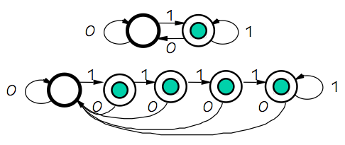 Equivalent FSMs
Consider the pair of FSMs diagrammed to the right: the 2-state ON/OFF switch
of the previous section, and a 5-state machine whose observable behavior is
identical to that of the two-state machine.
While consecutive presses of the $1$ button on the 5-state machine may cause
internal state changes among the four states for which the light is ON,
these four states are in fact externally indistinguishible. The only way
we could distinguish among these states is by opening the FSM and observing
internal state variables.
Definition (FSM equivalence): Two finite state machines are equivalent
if, for every finite input sequence, they produce identical output
sequences.
The notion of equivalent FSMs raises a practical optimization problem:
given an FSM $M$ that effectively serves some purpose, what is the simplest,
cheapest machine that is
equivalent to $M$?
There seems little point in paying for implementation complexity that
does not result in observable differences in behavior.
In fact, it is possible to recognise FSM equivalence and to systematically
reduce the complexity of an FSM to less complex equivalent machines.
Looking at the 5-state machine of this section, for example, one might
recognize that all of the four ON states are externally indistinguishible:
given the machine in one of these states, there is no sequence of inputs
we could enter to determine which of the ON states it was in.
Thus we suspect that three of the four ON states are redundant: we could
reduce the 5-state machine to the simpler 2-state equivalent machine
by merging the four ON states into one.
These notions lead to another, related, equivalence distinction:
Definition (state equivalence):
Two states $S_i$ and $S_j$ of a Moore FSM are equivalent if
(1) $S_i$ and $S_j$ produce identical outputs; and
(2) for every combination of inputs, $S_i$ and $S_j$ transition to equivalent states.
One approach to optimizing an FSM design is to repeatedly search for
and merge pairs of equivalent states, resulting in successively smaller
behaviorially equivalent machines.
One slightly bothersome detail in this
relaxation algorithm
is the
recursive
nature of our definition of state equivalence: if $S_i$ and $S_k$ transition
to different states $S_a$ and $S_b$ on some input $I$, we cannot conclude
that $S_i$ and $S_j$ are equivalent unless $S_a$ and $S_b$ are as well.
Indeed, if we begin with the conservatively pessimistic assumption that
states of our machine are distinct unless we can show their equivalence,
we may encounter situations where showning the equivalence of $S_i$ and $S_j$
reduces -- perhaps indirectly -- to showing the equivalence of $S_i$ and $S_j$.
Fortunately, this problem can be circumvented by starting our relaxation
(iteration) with the
optimistic assumption that every pair of
states is equivalent until shown otherwise by application of our state
(non)-equivalence definition.
In the 5-state example above, we quickly determine that the ON state cannot
be equivalent to any of the OFF states, but our deductions of non-equivalences
ends there, leaving us with the optimized 2-state equivalent FSM.
Example 2: Robotic Ant Controller
9.4. Example 2: Robotic Ant Controller
 RoboAnt
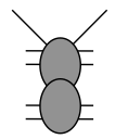
As a somewhat more entertaining example, we sketch in this section the
design of an FSM controller for the simple robotic ant shown to the left.
The sensory inputs to our ant controller are a single bit from each of two
antennae, which convey a $1$ only when the corresponding sensor is touching
a wall.
Our controller produces three outputs: $F$, which causes the ant to move
forward a small step during the next clock cycle, TL, causing slight turn to the left,
and TR causing a turn to the right.
Depending on these controller outputs, our ant will move or turn a small increment
during each clock cycle.
 RoboAnt Maze
Our goal is to make our ant smart enough to find its way out of a simple maze like that shown
on the right.
Our strategy is simple: we find a wall, and follow it using a "right antenna to the wall"
path which will eventually lead us to the outside. We assume that the turn and forward step
increments are small compared to the dimensions and 90-degree corners of the maze.
The ant will begin its quest by being placed at some arbitrary point
in the maze, neither antenna touching a wall, and with the controller
reset to its initial state.
 Lost
Lost
In this initial state, the ant is simply lost; its immediate goal is to
find a wall to follow to the exit.
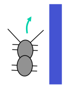
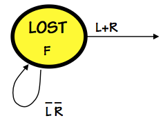 Initial state
To this end, we begin the design of our FSM with the initial state shown to the
right, in which the ant repeatedly steps forward until either its L (left) or R (right)
sensor reports a wall via a $1$ bit.
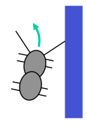
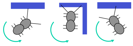 Wall encounter
When either or both antennae have touched a wall, we know that one of the three
situations shown on the left applies.
The ant responds to each of these situations by rotating counter-clockwise,
in an attempt to get into a configuration where the right antenna is not quite
touching a wall.
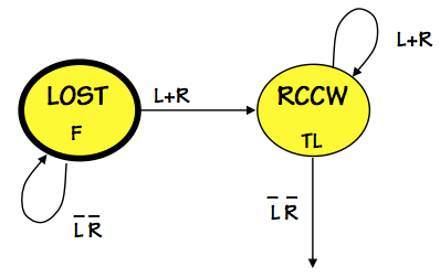 Rotate CCW
The $RCCW$ state does this by asserting the $TL$ output until neither
sensor reports a wall, at which point the ant is positioned to follow the wall to
its right.
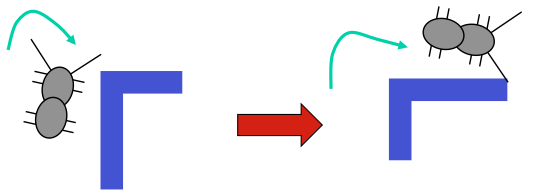
Given the single-bit input from our primitive ant's right sensor,
our strategy for following the wall to our right involves its intermittent
rather than continuous contact with the wall.
When the right sensor reports no wall as shown to the left,
we turn right and move forward in the hopes of re-establishing wall contact.
After turning sufficiently far that our sensor touches the wall,
we continue stepping forward but now turning left in an attempt to
move just beyond reach of the wall once again.
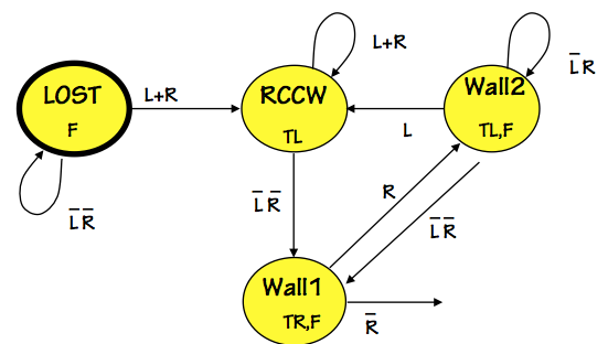 Wall-following states
This little ant dance is choreographed by two additionsl states named
$wall1$ and $wall2$.
Our controller alternates between these states, moving forward continuously
but oscillating between incremental right and left turns.
The $wall1$-$wall2$ pattern will continue so long as a straight
wall remains to the ant's right.
If this reverie ends by a frontal collision with a wall, both
sensors will report contact and the $RCCW$ state will be entered to
re-establish a path along the newly discovered wall.
An alternative disruption comes when the wall makes a sharp turn to
the right; in this case, we'd like our ant to follow the contour of the wall,
turning right until it re-established contact with the new wall surface.
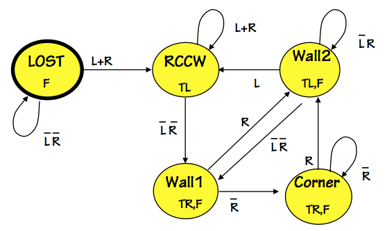 5-State Controller
We arrange this by adding a $corner$ state,
which steps forward and turns right until a wall is felt by the right antenna.
The resulting 5-state FSM is a workable first cut at our RoboAnt controller
design, and actually works well enough to allow our RoboAnt to find its way
out of an interesting variety of mazes.
Evolutionary step: equivalent state reduction
9.4.1. Evolutionary step: equivalent state reduction
Given our working 5-state RoboAnt controller, we might ask whether
there exists a simpler FSM with fewer states.
Given the notion of
state equivalence of
Section 9.3.2,
we might examine each pair of states in our 5-state machine to detect
equivalent -- hence redundant -- states in our design.
In this search, we can immediately rule out equivalence of any pair
of states that produce differing outputs.
Examining the 5 states of our controller design, this leaves only
one pair of states as candidates for equivalence: $Wall1$ and $Corner$,
both of which produce $TR,F$ as outputs.
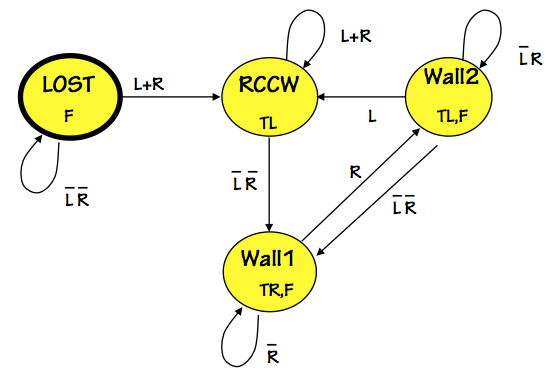 Equivalent 4-state FSM
Careful examination verifies that these two states transition to
identical (hence equivalent) states for each possible input,
leading us to conclude that the states are equivalent.
The equivalent states can be merged into a single state, leading to the
simplified 4-state FSM diagrammed to the left.
It is important to recognize that this 4-state version is equivalent
to the 5-state controller -- the behavior of the two machines is
externally indistinguishible.
However, the 4-state machine can be implemented using
two
bits of state variables rather than the three required for the
five-state version; moreover, a ROM-based implementation would
require a ROM of half the size.
This represents a substantial potential cost saving.
Chapter Summary
9.5. Chapter Summary
Finite state machines are an important conceptual model as well as
a practical engineering tool, and belong in the repertoire of every
digital systems engineer.
They encourage a view of memory as a set of
states rather
than
bits; the exponentially larger space of discrete states
parses stored information at higher resolution, often a useful
viewpoint.
Important facts about FSMs include:
- Moore machines are FSMs whose outputs depend only on current
state; outputs of Mealy machines reflect current inputs as well
as state.
- Implementation of an $N$-state FSM involves designing a digital
encoding for the $N$ states, typically using about $\log_2(N)$ flip flops.
Choice of state encoding can affect implentation cost and complexity.
- Equivalent FSMs produce identical output sequences
given identical input sequences; they are externally indistinguishible.
- Given a need for FSM $F$, it is generally useful to find the
simplest/cheapest FSM $F*$ to implement. A tool for this is
equivalent state reduction, by which redundant FSM states
can be identified and removed.