Synchronization and Arbitration
10. Synchronization and Arbitration
The engineering discipline introduced in
Chapter 8 allows us
to design sequential circuits that are provably reliable so long as setup
and hold time constraints -- our
dynamic discipline -- is adhered
to in the timing of input changes.
This powerful engineering tool allows us to build arbitrarily large clocked digital
systems from interconnected clocked components, but requires that the clocks
of the component systems be synchronized for the components to communicate
reliably. Where we can do so conveniently, we can satisfy the dynamic discipline
by using a single clock throughout the system.
However, it is not always convenient -- or even possible -- to guarantee
that inputs to a system are well behaved with respect to the system's clock;
Section 9.2.6 discusses one such common application.
These cases motivate us to explore the costs of
violating the
dynamic discipline, costs which are deceptively easy to underestimate
and have left several decades of scars on the history of digital systems
engineering.
One lesson from this chapter is the parallel roles of the
static
and
dynamic disciplines in our digital abstraction.
The former enables us to map continuous voltages into the discrete values of our
logic abstraction; its key feature is the exclusion of a range of voltages from
the mapping, to avoid requiring logic to make difficult distinctions between
voltages representing $0$ and $1$.
The dynamic discipline enables a similar continuous-to-discrete mapping,
but in the time domain.
It allows us to partition continuous time into discrete clock cycles,
reticulated by active clock edges.
Like the static discipline, it avoids difficult mapping decisions by
simply excluding a region of continuous time -- the setup and hold time
window surrounding each active clock edge -- from the mapping.
Thus these two cornerstone disciplines of our digital abstraction
move us into a world of discrete values as well as discrete time.
An Input Synchronizer?
10.1. An Input Synchronizer?
Section 9.2.6 sketches a common motivation for
dealing with asynchronous inputs, namely switch closures from
buttons pressed by a human user as shown to the right.
As the buttons may be pressed at arbitrary times, there
is no guarantee that their changes will avoid the stated
setup and hold time window specified by the clocked device.
Typically in such situations we can assume that the clock
frequency is fast with respect to button presses, and the
timing of each actual switch closure comes at a random point
during the clock cycle. If for example the clock period is
$100 ns$ and the total $t_s+t_h$ specification for the clocked
device is $10 ns$, we can expect that roughly $10$% of the
button presses will not obey the dynamic discipline and thus
potentially cause our clocked device to misbehave.
 Synchronizer
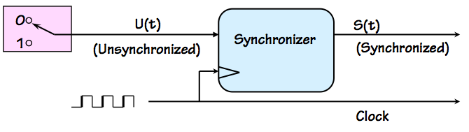
It is tempting to simply invent a fix in the form of a
synchronizer component, to be used wherever it
is necessary to deal with an asynchronous input.
The synchronizer takes a local clock signal as well as
an input $U(t)$ whose transitions are infrequent and asynchronous
with respect to the clock.
It produces, as output, a syncronous version $S(t)$ version
of the $U(t)$ input that is well-behaved with respect to the
clock: that is, $S(t)$ differs from $U(t)$ in that each transition
has been delayed to avoid a specified setup and hold time window
surrounding each active clock edge.
A workable synchronizer need only postpone troublesome
transitions in its input until they are safely distant from
active edges of the local clock. We can allow it to be
conservative about choosing to delay transitions, allowing it
to delay a few transitions that are just outside of the setup/hold
time window.
We can also be tolerant about the details of exactly when the
postponed transitions appear in the $U(t)$ output, so long as
they are synchronized with our clock; if our button press is
neglected for an extra cycle of our gigahertz clock,
the user is unlikely to notice. We might only require, for
example, that each output transition occur within $N$ clock cycles
of the corresponding input transition for some small constant $N$.
Given our tolerance for considerable sloppiness of this sort in
the specifications of a synchronizer, it seems entirely plausible
that such devices could be made to work reliably. Indeed,
there was a time when major companies included synchronizers
in their product lines.
The remarkable and painful lesson learned during recent decades,
however, is that synchronization is a much harder problem than
it seems.
It is, in fact,
impossible to build a perfectly
reliable synchronizer even given perfectly reliable components
of the sort that have been developed here.
The difficulty is that, given a transition $T_B$ in the synchronizer
input that is close to an active transition $T_C$ in the local
clock, our synchronizer must decide whether $T_B$ comes before $T_C$.
While our specifications allow the synchronizer's decisions to be
imperfect, we require them to be made in a bounded amount of time --
a constraint that is problematic for fundamental reasons.
The Asynchronous Arbiter
10.2. The Asynchronous Arbiter
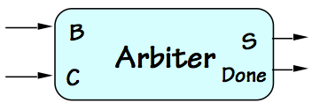
 Asynchronous Arbiter
The difficulty of knife-edge decision making in bounded time is
modeled by the specifications of a hypothetical device called
an
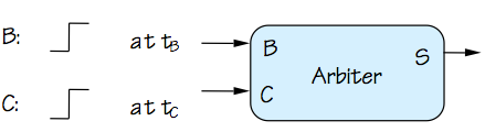
asynchronous arbiter, shown to the right.
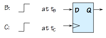
The device takes two digital inputs $B$ and $C$, each of which
makes a single $0 \rightarrow 1$ transition at times $T_B$ and
$T_C$ respectively.
The specifications for the arbiter involve
a finite
decision time $T_D$
and
a finite
allowable error $T_E$,
and specify that the value of the output $S$ at time $T_C + T_D$ must be
stable and valid no later than $T_D$ following the $T_C$ transition, and
its value after time $T_C + T_D$ must be
\begin{equation}
S = \begin{cases}
\mbox{valid 1}, & \mbox{if } t_B \lt t_C - t_E \\
\mbox{valid 0}, & \mbox{if } t_B \gt t_C + t_E \\
\mbox{valid 0 or 1}, & \mbox{otherwise}
\end{cases}
\end{equation}
Many varients of this specification capture the same basic idea:
the arbiter observes two asynchronous events, coded as positive
transitions on input signals, and -- after a finite propagation
delay $T_D$, reports which of the events came first.
Again, our specifications seem entirely reasonable from an
engineering standpoint: for close calls (events separated by
less than $t_E$ seconds) we'll accept
either decision
as to the winner; we do, however, demand an unequivocal decision,
in the form of a valid $0$ or $1$.
However reasonable our specification, it unfortunately cannot
escape the surprising truth:
For no finite
values of $T_E$ and $T_D$ is it possible to construct a
perfectly reliable arbiter from reliable components that
obey the laws of classical physics.
It took the digital community decades to accept this remarkable
fact, seduced as we were by the digital abstraction.
The difficulty, as we shall see, is the step of mapping a
continuous variable (like voltage or time) to a discrete
one
in bounded time, the fundamental problem
that motivates both our static and dynamic disciplines.
Note that this problem arises from the continuous variables
used in classical physics for underlying physical parameters;
there is a glimmer of hope that the problem might be
tractable using alternative models like quantum physics.
Naive Arbiter Implementation
10.2.1. Naive Arbiter Implementation
To the uninitiated, it might appear that an arbiter could be
implemented simply using a D flip flop.
 Isn't this an Arbiter?
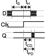
If we consider the application of our single-transition inputs to the D and clock
of a flip flop as shown on the right to be an arbiter whose decision time
is the flop's $t_{PD}$,
we can argue convincingly that
its Q output will conform to the arbiter specification when $t_B$
is sufficiently separated from $T_C$ that it falls outside of the
setup/hold time window. Indeed, the specifications for the flip
flop guarantee reliable operation so long as the dynamic discipline
is met; thus choosing the $T_E$ of the arbiter spec to be sufficiently
large as to cover the setup and hold times ensures that the device
will output valid $0$ when the arbiter is required to output $0$, and valid
$1$ when it is required to output $1$.
The only aspect of the arbiter spec that remains to be met is
that, when $t_B$ and $T_C$ are sufficiently close (within $t_E$
of each other), the arbiter must produce
either a valid
$0$ or a valid $1$. The value is completely arbitrary, but it
must be a valid logic level.
Although the allure of the digital abstraction tempts us to
assume that the flip flop output is valid outside of its
bounded-time transitions, that assumption turns out to be
a dangerous delusion.
In fact, we forfeit the promise of output validity following
a violation of the dynamic discipline by clocking an unsynchronized
input.
Although the problem encountered by this arbiter implementation
is fundamental to
any arbiter implementation, we
can gain some insight by diving in to see where our implementation
fails.
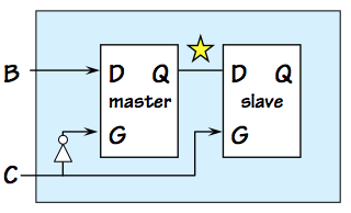
Recall that our D flip flop is constructed from two latches
as shown to the left, and that on an active (positive) clock
edge the slave "latches" a stored value that becomes the $Q$
output of the flop
as described in
Section 8.2.1.4.
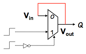
The latched value actually circulates around in a self-sustaining
cycle including a lenient multiplexor, as shown to the right
as the feedback path in red.
The other inputs to this multiplexor are such that the $V_{in}$ input
is amplified to produce the more valid $V_{out}$ output voltage.
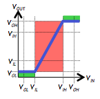
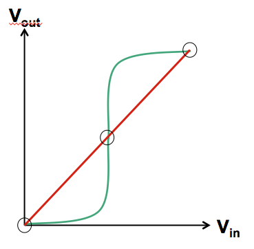
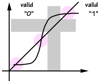
The voltage domain representation of the multiplexor's role in this
feedback loop is shown in green on the voltage transfer curve to the left,
while the $V_{in} = V_{out}$ constraint imposed by the red feedback path
is shown in red.
These two curves represent two equations constraining the $V_{in}$/$V_{out}$
of the latch producing the output voltage of our flip flop;
possible output voltages correspond to solutions to these simultaneous
equations, represented graphically by intersections of the red and
green curves.
We find three such intersections: two are the stable equilibria
that represent lached valid $0$ and $1$ logic values.
However, the geometry of our curves requires that there be a
third intersection between these two, the unstable equilibrium
often colloquially referred to as a
meta-stable state.
It represents a
fixed point of the positive feedback
path through the multiplexor -- an input voltage $V_M$ that
causes that path to generate an output that is also $V_M$.
Due to the continuity of the voltage transfer curve of the
multiplexor, such a $V_M$ always exists.
Typically $V_M$ is in the grey area between voltages which represent
valid logic levels, representing neither a valid $0$ nor
a valid $1$.
The bothersome metastable state is an inevitable consequence
of bistable behavior, and is exhibited by familiar examples from
our everyday lives.
We recognise as an unlikely but real outcome of coin flips
(landing on edge), horse races (dead heat), hockey games
(overtime), and other real-world decision-making processes.
The U.S. Presidential election of 2000 demonstrated that
the fundamental difficulty of bounded-time decision making
even extends to very large systems of arbitrary complexity.
The Metastable State
10.3. The Metastable State
We can observe several properties of the metastatble state:
- If the dynamic discipline is obeyed (by observing
flop setup/hold time constraints), the metastable state
will be reliably avoided. It becomes a problem only when
dealing with unsynchronized inputs.
- The metastable voltage $V_M$ represents the switching
threshold of our transistors, necessarily in the high-gain
region of their operation. For this reason, it is normally
not a valid logic level.
- The metastable state represents an unstable equilibrium:
a small perturbation in either direction will cause
it to accellerate in that direction, quickly settling
to a valid $0$ or $1$.
- The rate at which the output voltage $V_{out}$ of a flop
progresses toward a stable $0$ or $1$ value is
proportional to the distance between $V_{out}$ and $V_M$.
- Since $V_{out}$ is never exactly $V_M$,
$V_{out}$ will always settle to a valid $0$ or $1$
eventually.
- However, if $V_{out}$ may be arbitararily close to $V_M$,
it may take arbitrarily long for $V_{out}$ to become valid.
- The probabiliy of a flip flop remaining in a metastable
state for $T$ seconds falls off exponentially with $T$;
thus, simply waiting for a modest interval --
a clock cycle or two -- dramatically improves reliability.
Mechanical Analog
10.3.1. Mechanical Analog
 Mechanical Metastability
To gain some intuition about metastable behavior, let's
explore a simple hypothetical bistable mechanical
system.
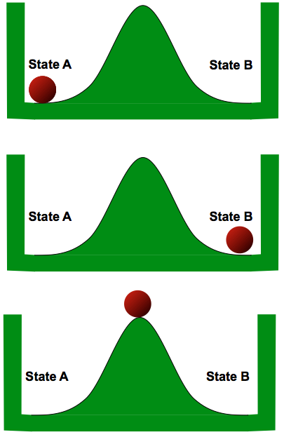
Consider a ball constrained to the confines of a deep well, whose
floor has a modest hill that separates local low spots on the left
and right sides of the well. Each of these low spots constitutes
a stable equilibrium position for the ball, as shown to the right;
however, there is an inevitable unstable equilibrium position at
the top of the hill.
The device is bistable. We could in principle use the position
of the ball -- left or right -- as a means to store a single bit,
and arrange to change the value of the stored bit by kicking the
ball to the left or right with enough force to reliably get it
to the opposite side of the hill.
Although we won't develop details of such a mechanical storage
device here, it should be quite plausible to the reader that
we could devise a way to make it work reliably.
Of course, there would be some rules that must be followed
for reliable operation; for example, one could not kick the
ball to the left and to the right at about the same time.
Such confusing instructions would compromise the momentum
imparted to the ball, and might result in the ball landing
near the unstable equilibrium point at the top of the hill --
the metastable state of our mechanical system.
Of course, given the vagueries of inaccuracies and noise, the
ball is never precisely at the metastable point; it
will always feel some slight force toward the left or the right.
It will always roll down the hill to one of the stable equilibria
eventually; but, depending on its distance from the metastable
point, this trip may take an arbitrarily long time.
Observable Metastable Behavior
10.3.2. Observable Metastable Behavior
One reason for the reluctance of the digital community to accept the inevitability
of arbitration failures is that they are inherently difficult to reproduce reliably
in the laboratory.
Even when violating the dynamic discipline by clocking unsynchronized data into
a flip flop at high frequencies, observable metastable behavior is quite rare:
it depends on pathological accidents of timing or other variables with precision
beyond our ability to control them reliably.
However, it is reasonably straightforward to devise an experimental setup
in which a flip flop is clocked repeatedly at high frequency, with a data
input whose transitions are timed so as to maximize the probability of
metastable failure.
 Typical observed metastable behavior
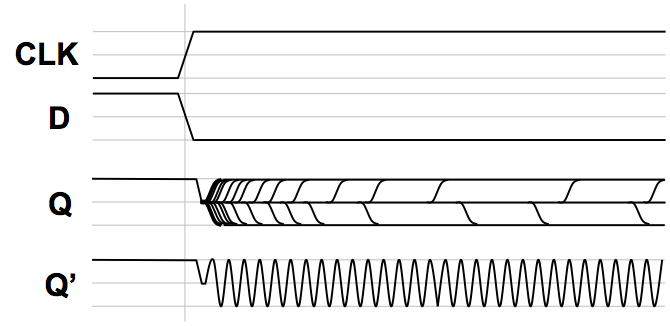
We might use an oscilloscope to observe many such experiments, resulting in
traces like those sketched to the right.
The top traces of this image show the clock and D inputs to our test flip flop,
making transitions at about the same time.
The value labeled $Q$ shows the superposition of the output trace over many consecutive
clock cycles.
Note that in this family of traces, $Q$ assumes three dominant values:
valid $0$, valid $1$, and the metastable voltage between the two.
Following an active clock edge $Q$ moves to the metastable voltage,
where it persists for a variable period before eventually snapping to a
valid $0$ or $1$ value.
It should be noted that many other observable symptoms of arbitration
failure are possible.
Once we violate the dynamic discipline, there are
no guarantees
about the value circulating around our combinational feedback loop.
The multiplexor input is invalid, so it need not produce a valid output.
Rather than settling to the metastable voltage, for example, the value
circulating might exhibit high-frequency oscillation such as that shown
as $Q'$. Depending on parasitic reactive components in the feedback
loop, such dynamic invalidity is sometimes observed.
Delay and Validity Probability
10.4. Delay and Validity Probability
We have already noted that problems with metastability can be avoided
simply by assuring that the dynamic discipline is followed by our
clocked circuits -- specifically, that input signals to each clocked
component are valid and stable during that component's specified
setup/hold time window.
Although the problem is fundamental when an unsyncronized input must
be passed to a clocked system, metastable behavior and its consequent
system failures are still quite rare.
 Synchronizer test setup
Consider clocking a single unsynchronized transition into a
flip flop whose setup and hold time are $t_S$ and $t_H$, respectively,
and whose clock period is $t_{CLK}$.
The probabability that an instantaneous transition will fall
within the forbidden setup/hold time window,
a prerequisite condition for arbitration failure, is thus $(t_S+t_H) / t_{CLK}$.
This value represents a crudely pessimistic upper bound on the probability
of a failure, and suggests that minimizing the $t_S+t_H$ window (by
use of high-gain devices in our flip flop design) decreases
probability of arbitration failures.
It also implies that the problem is exacerbated by a high clock
frequency.
Probability of nearness to metastable point
10.4.1. Probability of nearness to metastable point
In fact, metastable behavior is exhibited only when pathological
input timing leads to a circulating voltage that is very close to
the metastable value $V_M$.
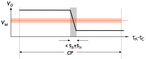
While a precise mathematical model for the circulating voltage $V_0$ immediately
following an active clock edge is complex, we can again make the
very conservative (pessimistic) assumption that it varies linearly
between valid logic levels over the forbidden $t_S+t_H$ time window
as represented by the black line in the graph above.
In fact, problems occur only when this voltage falls near the metastable point,
shown above as a narrow colored band centered on $V_M$.
Using this model, we can approximate the probability that $V_0$ -- the
circulating voltage immediately following the clocking of an unsynchronized
input -- falls within $\epsilon$ of the metastable voltage as
\begin{equation}
Pr[ | V_0 - V_M | \leq \epsilon ] \leq { ( t_S + t_H ) \over t_{CLK} } * { {2 \cdot \epsilon} \over ( V_H - V_L ) }
\label{eq:prob_within_epsilon}
\end{equation}
Delay cures metastability
10.4.2. Delay cures metastability
Near the metastable point, our feedback loop amplifies the
distance between the circulating voltage $V$ and the metastable
point $V_M$, by moving $V$
away from $V_M$ at a rate
proportional to $V - V_M$.
The constant of proportionality $A$ is a function of circuit details like
the amplification (gain), as well as the parasitic resistance and
capacitance of the circuit.
You may recognize this pattern -- rate X changes proportional to X --
as a formula for exponential growth, and indeed the trajectory of $V$
away from the metastable voltage is described by
\begin{equation*}
V - V_M \approxeq \epsilon \cdot e ^ { { T / \tau }}
\end{equation*}
in the vicinity of the metastable point,
where $\epsilon$ is the starting distance $|V_0 - V_M|$ and $\tau$ is a
time constant dependant on circuit parameters.
Given this model for the rate at which the circulating voltage $V$
progresses
away from the troublesome metastable value,
we can approximate the amount of time it will take for $V$ to progress
from a value near $V_M$ to a valid $0$ or $1$. We do this by a
formula that specifies, for a given time interval $T$, how close
$V_0$ must be to $V_M$ to require $T$ seconds for $V$ to become
valid:
\begin{equation*}
\epsilon ( T ) \approxeq (V_H - V_M) \cdot e ^ {-T / \tau}
\end{equation*}
Together with equation \eqref{eq:prob_within_epsilon}, we can
approximate the probability that the output of our synchronizer
flop remains invalid $T$ seconds after clocking an unsynchronized
input as
\begin{equation*}
Pr_M(T) \approxeq Pr[ |V_0 - V_M| < \epsilon ( T ) ]
\approxeq K \cdot e ^ {- T / \tau }
\end{equation*}
where $K$ and $\tau$ are constants derived from implementation parameters.
While we have glossed over a variety of issues in arriving at this
formula, it underscores an important observation about the metastable
behavior that causes synchronization failures: the probability that
a flipflop output will remain invalid decreases
exponentially
with elapsed time.
This key fact allows us an engineering workaround, which reduces the
unsolvability of the arbitration problem from a showstopper to an
annoyance: we can, in fact, clock unsynchronized inputs to an
arbitrarily high level of reliability by simply introducing modest delay
for any metastable behavior to settle.
| | Average time |
|---|
| T | $Pr_M(T)$ | between failures |
|---|
| $31$ ns | $3 \cdot 10^{-16}$ | $1$ year |
| $33.2$ ns | $3 \cdot 10^{-17}$ | $10$ years |
| $100$ ns | $3 \cdot 10^{-45}$ | $10 ^ {30}$ years |
To appreciate the scale of the delays involved,
the table to the right shows some failure probabilities computed using
conservative values from decades-old process parameters. While the
actual numbers are of little relevence, it is noteworthy that the
exponential relationship between delay and settling time yields
astronomically high reliability rates from modest delays.
You may recall that the age of the earth is estimated to be on
the order of $5 \cdot 10^9$ years, making the failure rates
attainable at the cost of tens of nanoseconds delay seem quite
acceptable.
Bounded-time Discrete Mapping
10.5. Bounded-time Discrete Mapping
The problem of making
"which came first?" decisions in bounded time
confronted by the arbiter is, in fact, an instance of a more general
difficulty: the problem of mapping a discrete variable into a
continuous one.
If the mapping is nontrivial (in the sense that its range includes multiple
discrete values), there will be input values $i_1$ and $i_2$ that map
to distinct discrete outputs $V_1$ and $V_2$, respectively.
If the mapping is to be performed by a mechanism that computes
$V = f(i)$ for some continuous function $f$, the continuity of $f$
assures that there will be input values between $i_1$ and $i_2$ that
produce output values between $V_1$ and $V_2$.
Indeed, even if $f$ has a discontinuity for some input $i_1 < i_M < i_2$,
the mapping of $i_M$ is ambiguous and hence problemmatic.
We have seen this problem in the mapping of continuously-variable voltages
to discrete $1$s and $0$s in
Chapter 5,
where we conspired to avoid the difficult decision problems by
an engineering discipline that excludes a range of voltages from
our mapping and avoids requiring our circuits to interpret these
values as valid logic levels.
When we moved to discrete time in
Chapter 8,
we introduced an analogous discipline to duck hard problems
deciding the ordering between active clock edges and input
data transitions.
In this case, our excluded "forbidden zone" is the range of continuously
variable timing relationships ruled out by the setup/hold time window
of the dynamic discipline.
What we cannot do reliably
10.5.1. What we cannot do reliably
The difficult problems identified in this chapter share the attributes
that they involve a
nontrivial continuous-to-discrete mapping that
must be made in
bounded time.
If we relax either of these constraints, solutions become plausible.
The astute reader might recognise that this is is essentially the
same problem, translated to the time domain, that was addressed in the
voltage domain in
Chapter 5 by the forbidden
zone and noise margins.
The static discipline avoids unbounded-time decisions about whether
a continuously variable voltage represents a $1$ or a $0$;
the dynamic discipline avoids
unbounded-time decisions about whether a clock transition at $t_C$
comes before a data transition at $t_D$.
Each of the avoided problems involves a mapping of a continuous
variable into two discrete cases: in the former case the variable
is a voltage, in the latter a time interval $t_C - t_D$.
We have already seen that the asynchronous arbiter, which decides the
ordering of two transitions within a finite propagation delay following
either (the first, the last, or a specific input) cannot be reliable
if its implementation follows the continuous mathematics of classical
physics; this fact remains true even if we allow it to report an arbitrary
result in close cases.
The synchronizer of
Section 10.1 is a minor
variant of the arbiter, and suffers similar unreliability issues.
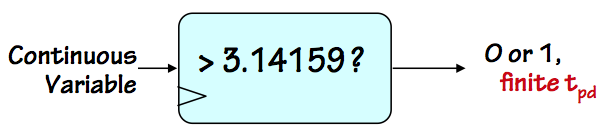
Other continuously variable inputs also resist knife-edge decisions in bounded
time.
Consider a module that compares an input voltage to a fixed threshold, reporting
if the input is above or below the threshold value.
Even if we allow it to be wrong in close cases, this
analog comparator
cannot make a decision in bounded time; again, this confronts the
fundamental difficulty of a bounded-time continuous-to-discrete mapping.
What we CAN do reliably
10.5.2. What we CAN do reliably
Although nontrivial bounded-time mapping of continuous to discrete variables
confronts fundamental problems,
slight relaxation of critical problem constraints makes seemingly close relatives
tractible.
Perhaps the most obvious solvable variant is our clear ability to make
a reliable device that performs a
trivial mapping of continuous
to real values in bounded time.
A device implemented by a connection to ground, for example, could
reliably report that $T_B < T_C$ for
any relative timing of
two transitions, or that $V < 3.14 volts$ for any input voltage $V$.
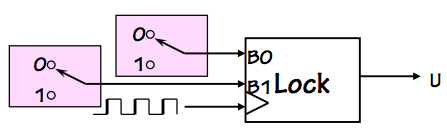
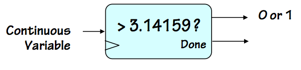
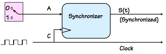
A more interesting example is an
unbounded-time arbitor such as the one
shown to the left.
Rather than requiring that this device produce a valid $S$ output within a
prescribed $t_{PD}$, it is allowed to take any (finite) interval to make its
decision, and signal (via a $Done$ output) when its decision is made.
Given reasonable specifications (include a range of input timings for
which either answer is acceptable), this device can operate
reliably.
Similarly, an
unbounded time analog comparator can in principle be made
to work reliably.
Again, a finite range of allowable errors must be provided for in its specification.
Although bounded-time
which-came-first decisions are hard,
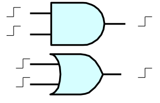
certain functions of signals with asynchronous transitions are straightforward.
Consider a 2-input device which signals an output a finite period after
the second of two input transitions has occurred; can such a device be made
reliable? How about signaling shortly after the
first of the two transitions?
These specifications are nicely met by combinational AND and OR gates.
Folk Cures
10.5.3. Folk Cures
The fundamentals of synchronization and arbitration failures
have taken decades to be accepted by the engineering community.
This history is laced with interesting proposed "solutions"
to the problem of building a reliable synchronizer, most of
which can be viewed with the same skepticism we might apply
to a new proposal for a perpetual motion machine.
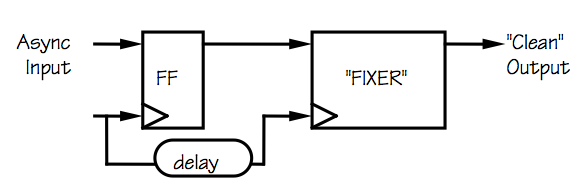
One class of naive proposals involves a
fixer module that
can be spliced into specific circuit locations that are experiencing
synchronization failures, such as that shown to the right.
The input to the fixer module is a potentially invalid logic level,
such as the output from a flip flop clocking an asynchronous input.
The fixer is supposed to detect whether its input is a valid logic
level and correct it (to a valid level) if it is invalid, all
within a bounded time interval.
While there are many things wrong with such proposals, one that
is obvious in the restrospect of decades of recent history is that
the problem of deciding whether a given voltage is valid cannot itself
be solved in bounded time.
Once again, this decision represents a nontrivial mapping of a continuous
variable (input voltage) to a discrete one (validity); there will always
be an input value that will produce an output halfway between true and false.
One particularly creative class of proposals involves eliminating the
problem by an auspicious manipulation of our definitions of logical
validity.
While accepting the need for noise margins and forbidden zones
in our mapping of voltages to valid logic levels discussed in
Chapter 5, it is not actually required
that the metastable fixed-point voltage $V_M$ of a flip flop
fall in the forbidden zone.
We might devise a logic family, for example, where the
metastable voltage is deemed a valid $0$.
In this family, a flip flop that clocks an unsynchronized
input may still hang at the metastable voltage for an arbitarily
long interval; but now its output will be a valid $0$ during
that interval.
The downside of this approach?
After clocking an unsyncronized input, a flip flop whose output
is metastable (producing what is now interpreted as a valid $0$)
will eventually progress to a valid logic level.
About half the time, it will choose to emerge from the metastable
state to become a valid $1$.
In our new logic family, this will be seen by surrounding logic as
a spontaneous transition of the flop output from $0$ to $1$ -- a
behavior not likely to be appreciated by the circuit designer.
Dealing with Asynchronous Inputs
10.6. Dealing with Asynchronous Inputs
The fundamental difficulty associated with clocking asynchronous signals
is an accepted fact among the modern engineering community.
Failure to obey the dynamic discipline creates a finite probability
of an invalid logic level in our digital system.
One invalid signal may stimulate others: the static discipline
guarantees valid outputs from valid inputs, but guarantees
nothing for
invalid inputs.
In principle, a requirement to accept asynchronous inputs threatens
the integrity of our digital system engineering discipline.
Once understood, however, the practical impact of the synchronization
problem is modest.
Keys to our coping with asynchrony include the following:
- Synchronize clocks:
Avoid the problem where possible, by using a single
clock discipline or synchronizing the clocks of separate
subsystems that must communicate.
- Delay:
Where asynchronous inputs cannot be avoided, allow
sufficient delay for the output of the synchronizing
flip flop to settle that the probability of failure
is acceptably low.
The exponential decay of failure probability with delay
interval reduces the problem of failure to a fairly modest
cost in latency.
- Hide delay:
Under certain circumstances, enginnering tricks can be used
to eliminate some or all of the delay by predicting
arbitration problems and solving them in advance of the
actual input event.
The first of these guidelines simply reflects the fact that
there is a cost associated with synchronization of input data,
and that synchronization problems shouldn't be casually introduced
-- for example, by needless use of multiple unsynchronized clocks
in different parts of a system.
While there are circumstances where a multiclock system makes sense,
such a system is carefully partitioned into several
clock domains
and special care given to communication between the domains.
The second guideline reflects our recognition that we can reduce
the probability of failure to an arbitrarily low level by adding
modest delay.
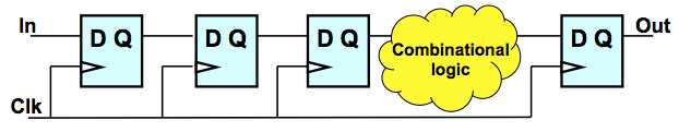
Often one sees a configuration such as that shown to the right,
forcing an input signal to pass through multiple, apparently redundant,
flip flops.
This pattern represents an effective way to convert an asynchronous input
to a derived synchronous signal whose probability of invalidity
$t_{PD}$ after an active clock edge is acceptably small.
A common informal analysis of this circuit reasons that
if the probability that the output of the leftmost flop is
invalid is some small number $p$,
the probability of invalidity at the output of the flop to
its right is $p ^ 2$, $p^3$ at the third flop, etc.
While there may be some merit to this reasoning,
the more general principle is the exponential falloff
of failure probability with delay outlined in
Section 10.4.2.
Each flop the signal passes through delays its entering
subsequent circuitry by a clock cycle, and consequently
enhances its reliability by a large factor.
Under most circumstances, the delay of an asynchronous input
by a few clock cycles reduces failure probability to a
ridiculously low level with negligible impact on the
function or performance of the system.
In latency-sensitive applications, however, the delay
required for reliable communication may compromise performance.
In these cases, it may be worth exploring some special-case
optimizations suggested by the third of our guidelines.
For example, communication between digital subsystems
that require different frequency clocks might be made reliable
if one clock period is a multiple of the other that
maintain a fixed synchronous relationship.
This idea may be generalized to deal effectively with clocks
whose periods have the ratio $m/n$ for various integral $m$ and $n$.
1
The predictablity of the timing of active clock edges in such cases
allows the generation of a "scrubbed" version of the local clock
for use in clocking in asynchronous data.
The scrubbed clock omits active clock edges that come at
dangerous times.
While this decision -- whether a given clock edge is dangerous --
is itself an abitration problem, it can be performed beforehand
in real time or even precalculated and wired into the design.
In general, any known constraints on the timing of the incoming
asynchronous input can be exploited -- at some engineering cost --
to reduce or eliminate the delay needed to reliably communicate.
Further Reading
10.7. Further Reading
Chapter Summary
10.8. Chapter Summary
Synchronization failures have played an unexpectedly significant role
in the history of digital engineering, likely due in large part to
the conceptual appeal of the digital abstraction.
Digital engineers, seduced by the comfortable world of $1$s and $0$s,
have demonstrated a remarkable resistance to the notion that the cost
of violating the dynamic discipline is abdicating the guarantee of
validity. And once any invalid signal creeps into our system, it
can propagate elsewhere: the "valid in $\rightarrow$ valid out"
construction rule no longer prevents logically invalid levels.
Important facts to understand and remember:
- Synchronization failure is a problem only when the dynamic
discipline is violated, e.g. by an input that changes asynchronously.
- Every bistable storage device has, in addition to the two
stable equilbria used to represent its two possible values, a
third unstable equilibrium called the metastable state.
Without constraints on the timing of input changes (the dynamic
discipline), the bistable device may enter this state,
resulting in invalid output values;
- Metastable behavior eventually resolves to a valid $1$ or $0$,
but the time required is unbounded.
- The probability of metastable behavior persisting for $t$ seconds
falls off exponentially with $t$, so a modest delay after an unsynchronized
input can reduce the probability of invalid outputs to be negligible.
- Synchronization failures are best avoided by
- Avoiding asynchronous inputs where possible; and
- Allowing sufficient delay after clocking unavoidably
asynchronous inputs.
The primary practical impact of these issues is the acceptance by
the digital engineering community of modest delay as a fundamental
cost associated with asynchronous inputs.